This class was devoted to an informal discussion of the topics we plan to cover this semester. We began by describing the type of functions we will study, namely scalar valued and vector valued functions of several variables. We illustrated, in a general way, how with the proper definitions, many of the basic concepts from Calculus I and Calculus II can be extended to functions of several variables. On the other hand, we noted, for example, that for a function of two variables, one can measure a rate of change in infinitely many different directions, something not encountered in Calculus I.
We then gave a brief overview of how the integration process works in general: One always has a function to integrate (the integrand) and a domain of integration. We then described how the integration process works in all scenarios we will encounter during the semester. Namely, starting with a domain of integration and a function defined on that domain, we proceed as follows:
- (i) Subdivide the domain of integration into small portions of a similar type, e.g, if the domain of integration is a solid, subdivide into smaller solids; if the domain of integration is a curve, subdivide into smaller curves. One can assume the individual portions have the same size.
- (ii) Choose a point in each subdivision and evaluate the function at that point.
- (iii) Multiply the answer in (ii) by the size of the subdivision, e.g., volume if a solid, length if a curve.
- (iv) Add the quantities in (iii).
- (v) Take the limit of the sums in (iv) as the size of the subdivisions tend to zero.
We continued our discussion of functions of several variables, with the examples (like, though not exactly) \(f(x,y)= x^2+y^2\), \(g(x,y,z) = \frac{1}{x^2+y^2+z^2}\), and \(h(x_1, x_2, \ldots, x_n) = x_1+x_2+\cdots+x_n\). We noted that \(f(-2, 3) = (-2)^2+3^2 = 13\), \(g(1,2,3) = \frac{1}{1^2+2^2+3^2} = \frac{1}{14}\), and \(h(1,2,\ldots, n) = 1+2+\cdots +n = \frac{n(n+1)}{2}\).
We then noted that the range and domain for functions of several variables, have the same meaning as for functions of a single variable, namely the domain is the set of allowable inputs and the range is the set of possible outputs. In the case of a function of two variables, say, the allowable inputs will elements of \(\mathbb{R}^2\), but the the outputs are always real numbers. For the functions defined above, we have:
- (i) \(f(x,y):\) Domain = \(\mathbb{R}^2\) and range = \(\{\alpha\in \mathbb{R}\ |\ \alpha\geq 0\}\).
- (ii) \(g(x,y,z)\): Domain \(\mathbb{R}^3\backslash (0,0,0)\) and range = \(\{\alpha \in \mathbb{R}\ |\ \alpha > 0\}\).
- (iii) \(h(x_1, x_2,\ldots, x_n)\): Domain = \(\mathbb{R}^n\) and range = \(\mathbb{R}\).
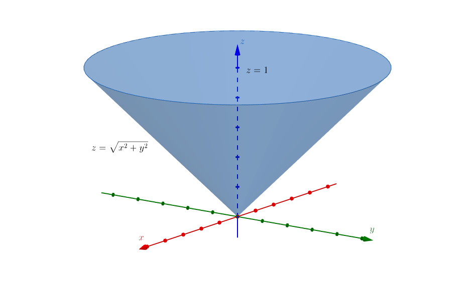
One notes that for the function \(t(x,y) = \sqrt{1-x^2-y^2}\), the domain is the the unit circle of radius one centered at the origin in \(\mathbb{R}^2\) and its interior, while the range is \(\{\alpha\in \mathbb{R}\ |\ 0\leq \alpha\leq 1\}\). After this we discussed graphing functions of two variables \(z = f(x,y)\) and how the level curves \(f(x,y) = c\) for different values of \(c\) help to understand the graph of \(f(x,y)\). We also cautioned that the level curves do not give a complete picture of the graph, since for example, the level curves of \(f(x,y) = x^2+y^2\) and \(g(x,y) = \sqrt{x^2+y^2}\) are circles of increasing radii, as \(c > 0\) increases, but the graph of \(f(x,y)\) is a paraboloid ( see here) while the graph of \(g(x,y)\) is a cone ( see here). We noted that the difference between these two surfaces can be seen by taking curves obtained by setting \(y = c\), and in particular \(y = 0\). In this cross section, the graph of \(f(x,y)\) is a parabola while the graph of \(g(x,y)\) is the graph of \(z = |x|\) in the \(xz\)-plane, i.e., two rays emanating from the origin at 45 degrees.
We began a discussion of limits and continuity for functions of several variables. As a reminder, we first discussed the concepts of limit and continuity, for a function of one variable. Just as \(\lim_{x\to a}f(x) = L\) intuitively mean that the values of \(f(x)\) approach \(L\) as \(x\) approaches \(x\), it should be the case that \(\lim_{(x,y)\to(a,b)} f(x,y) = L\) means that the values of \(f(x,y)\) approach the real number \(L\), as \((x,y)\) approaches \((a,b)\). We noted that while limits for functions of one variable involve \(a\) approaching \(x\) from either the right or left, for limits with functions of two variables, there are infinitely many ways \((x,y)\) can approach \((a,b)\). On the other hand, using the notion of distance, the definition of a limit still takes a very similar form as in one variable: Namely, we say \(\lim_{(x,y)\to (a,b)} f(x,y) = L\) if for every \(\epsilon > 0\), there exists \(\delta > 0\), such that \(|(x,y)-(a,b)| < \delta\) implies \(|x-L| < \epsilon\). We then defined \(f(x,y)\) to be continuous at \((a, b)\) if \(\lim_{(x,y)\to (a,b)} f(x,y) = f(a, b)\).
Before calculating some examples, we noted that the following rules for taking limits hold, and that these are the same rules that apply when taking limits of function of one variable.

Thus, for example,
We also noted that when applying the rules above to \(\lim_{(x,y)\to (a,b)} f(x,y)\) it is crucial to use limits, and not merely substitute \((a,b)\) for \((x,y)\). For example, let
so that \(\lim_{x\to 3} a(x) = 1 ,\not = 2\) and \(b(y) = 2y\). Then for \(f(x,y) = a(x)b(y)\), we have \(\lim_{(x,y)\to (3,2} f(x,y) = 1\cdot 4 = 4\).
We then noted that the same rules above for limits apply for continuity, e.g., sum, products etc of functions continuous at \((a,b)\) are continuous at (a\(,b)\). We finished class by first showing \(\lim_{(x,y)\to (0,0)} f(x,y)\) does not exist, for \(f(x,y) = \begin{cases} \frac{x^2-y^2}{x^2+y^2}, \ if\ (x,y) \not = (0,0)\\0\ if\ (x,y) = (0,0).\end{cases}\) and discussing an approach for evaluating the limit \(\lim_{(x,y)\to (0,0)} f(x,y)\) for \(f(x,y) = \begin{cases} \frac{3x^2y-y^3}{x^2+y^2}, \ if\ (x,y) \not = (0,0)\\0\ if\ (x,y) = (0,0)\end{cases}\) using trigonometric substitution with \(x = r\cos(\theta)\) and \(y = r\sin(\theta)\).
We reviewed the definitions of limit and continuity for scalar functions of the form \(f(x,y)\). After doing an example where the function was continuous so that the limit was obtained by substitution, we considered the following limit: \(\lim_{(x,y)\to(0,0)} \frac{4xy^2}{x^2+3y^4}\). We noted that the limit was zero as \((x,y)\) approached (0,0) along any line \(y = kx\), for \(k\in \mathbb{R}^2\), but that the limit is not zero as \((x,y)\) approached (0,0) along the curve \((y^2, y)\). This shows that for \(\lim_{(x,y)\to (a,b)} f(x,y)\) to exist, it is not just a matter of the limit existing as \((x,y)\) approached \((a,b)\) from all possible directions.
We then worked through an \(\epsilon, \delta\) proof of the two facts: (i) \(\lim_{(x,y)\to (a,b)} x = a\) and (ii) The limit of a sum is the sum of the limits.
We ended class by discussing limits and continuity for vector valued functions \(F : \mathbb{R}^n \to \mathbb{R}^m\), noting that the concept of distance renders the corresponding definitions almost identical to the case of \(f(x,y)\) previously discussed: For \(P\in \mathbb{R}^n\) and \(L \in \mathbb{R}^m\), writing \(\underline{x}\) for \((x_1, \ldots, x_n)\), we have \(\lim_{\underline{x}\to P} F(\underline{x}) = L\) if for every \(\epsilon >0\), there exists \(\delta > 0\) such that \(||F(\underline{x})-L|| < \epsilon\), whenever \(||(\underline{x})=L|| < \delta\) and, moreover, \(F(\underline{x})\) is continuous at \(P\) if \(\lim_{\underline{x}\to P} F(\underline{x}) = F(P)\). We then stated the theorem that if
We began our discussion of partial derivatives. We noted that given a function \(f(x,y)\), if we start at the point \((a,b)\), then there are infinitely many directions moving away from \((a,b)\) for which we could seek the rate of \(f(x,y)\). Our analysis began with the rate of change of \(f(x,y)\) at \((a,b)\) in a direction parallel to the \(x\)-axis. We noted that this can be analyzed by intersecting the graph of \(z = f(x,y)\) with the plane \(y = b\). We observed that doing so reduces the problem to calculating the derivative of the function \(c(x) := f(x,b)\) at \(x = a\). Thus,
If this limit exists, this is the partial derivative of \(f(x,y)\) with respect to \(x\) at \((a,b)\), which we denote by \(\frac{\partial f}{\partial x} (a,b)\) or \(f_x(a,b)\). Geometrically, we can think of \(\frac{\partial f}{\partial x}(a,b)\) as the slope of the line passing through the point \(a,b, f(a,b)\) tangent to the curve \(z = f(x,b)\) lying on the graph of \(z = f(x,y)\).

We then used the limit definition to calculate \(f_x(1,1)\) for the function \(f(x,y) = 2x+3y\) and \(g_x(2,-1)\) for the function \(g(x,y) = x^3y+3xy^2\). The resulting values were 2 and -9. We then repeated the limit calculations to find the general values of \(f_x(x,y)\) and \(g_x(x,y)\), and observed that \(f_x(x,y) = 2\) and \(g_x(x,y) = 3x^2y+3y^2\). This suggests that in general, when the relevant limits exist, the partial derivative of an arbitrary \(f(x,y)\) with respect to \(x\) is obtained by differentiating the expression for \(f(x,y)\) with respect to \(x\), treating \(y\) as a constant. We then did this direct calculation for \(h(x,y) = 6x^2y^3e^{x^2+2y^2}+5\cos(xy)\), obtaining
We then noted that the discussion above applies equally well to the variable \(y\), so that one defines the partial derivative of \(f(x,y)\) with respect to \(y\) at \((a,b)\) as

Accordingly, the function \(\frac{\partial f}{\partial y}\) is calculated by differentiating \(f(x,y)\) with respect to \(y\), treating \(x\) as a constant. Doing so for \(h(x,y)\) above yields,
We ended class by noting that the following rules for partial differentiation (and their more general counter parts) follow from the corresponding familiar rules from Calculus 1.
For functions \(f(x, y)\), \(g(x,y)\), \(h(t)\) :
- (i) \((f+g)_x = f_x+g_x\)
- (ii) \((fg)_x = f_xg+fg_x\)
- (iii) \(h(f(x,y)_x = h'(f(x,y)) \cdot f_x(x,y)\),
We began class reaclling the partial derivatives of functions of two variables and noted that the definition easily carries over to functions of several variables, the general case being a function \(f(x_1, x_2, \ldots, x_n)\). In this case, we defined the partial derivative of \(f(x_1, \ldots, x_n)\) with respect to \(x_i\) at \((a_1, \ldots, a_n)\) to be
if the limit exists. We then noted that to calculate partial derivatives of functions of many variables with respect to a given variable, we differentiate with respect to that variable, treating all remaining variables as constants. We then calculated the partial derivatives of the function \(f(x,y,z,w) = x^2y^3z^4w^5+e^{xy+zw}\).
We then began a discussion of finding the tangent lines to the graph of \(z = f(x,y)\) in the \(x\) and \(y\) directions at the point \(a,b,f(a,b)\), using the fact that for the function \(f(x,y)\), if \(f_x(a,b)\) exists, \( f_x(a,b)\) as the slope of the line passing through the point \(a,b, f(a,b)\) tangent to the curve \(z = f(x,b)\) lying on the graph of \(z = f(x,y)\) in the plane \(y = b\). From this, were able to derive the parametric equation for this line:
We then noted that having good tangent lines in two directions leads to the expectation of having a tangent plane at the point \(a,b, f(a,b)\). We ended class by recalling the fact that if \(P = (a,b,c)\) is a point on the plane \(F\) and \(\vec{n} = (n_1,n_2,n_3)\) is normal to \(F\), then the equation of \(F\) is the set of all points in \(\mathbb{R}^3\) satisfying \(0 = n_1(x-a)+n_2(x-b)+n_3(z-c)\).
We began class by recalling the parametric equations of the tangent lines in the \(x\) and \(y\) directions to the graph of \(z = f(x,y)\) at the point \(a,b, f(a,b)\). We then noted that having good tangent lines in two directions leads to the expectation of having a tangent plane at the point \(a,b, f(a,b)\). After recalling the fact that a plane is determined by a point and a normal vector, we arrived at the equation for what should be the relevant tangent plane:
Definition. Given \(f(x,y)\) and \((a,b)\) in the domain of \(f(x,y)\). Suppose that \(f_x(a,b)\) and \(f_y(a,b)\) exist and set \(L(x,y) := f_x(a,b)(x-a)+f_y(a,b)(y-b)+f(a,b)\). Then \(f(x,y)\) is differentiable at \((a,b)\) if
- (i) The function \(L(x,y)\) is a good linear approximation to \(f(x,y)\) for points \((x,y)\) sufficiently close to \((a,b)\).
- (ii) The proposed tangent plane \(z = L(x,y)\) is, in fact, tangent to the graph of \(f(x,y)\) at \((a,b)\).
We finished class by showing directly that \(f(x,y) = xy\) is differentiable at \((a,b)\), for all \((a,b)\in \mathbb{R}^2\).
We began class by reviewing the definition given in the previous lecture regarding the differentiability of \(f(x,y)\) at \((a,b)\), noting \(L(x,y)\), as previously defined, is a good linear approximation to \(f(x,y)\) at \((a,b)\). Geometrically, this means that there is a well defined tangent plane to the graph of \(z = f(x,y)\) at \(a,b, f(a,b)\). In other words, does the proposed tangent plane
We then stated the following very important theorem:
Theorem. (Differentiability Criterion) Given \(f(x,y)\) and \((a,b)\) in the domain of \(f(x,y)\) and suppose \(f(x,y)\) has the property that \(f_x(x,y)\) and \(f_y(x,y)\) exist and are continuous in an open disk about \((a,b)\). Then \(f(x,y)\) is differentiable at all points in that disk, including the point \((a,b)\). Here an open disk of radius \(r\) about \((a,b)\) means the set of points in \(\mathbb{R}^2\) whose distance from \((a,b)\) is less than \(r\).
To illustrate the connection between the conditions in the theorem, we considered two examples. First we looked at \(f(x,y) = ||x|-|y||-|x|-|y|\) and then \(f(x,y) = \frac{2xy}{\sqrt{x^2+y^2}}\). In both cases we saw that both partials exist at (0,0), but that the function is not differentiable at (0,0). In each case the failure of differentiability was due to the fact that the partial derivatives are not continuous at (0,0).
We then noted that if \(f(x,y)\) is differentiable at \((a,b)\) and \(\Delta x\) and \(\Delta y\) are small, then
We then illustrated this with the following example.
Example. Use the linear approximation to estimate \(f(1.01, 2.02)\), for \(f(x,y) = x^2+2xy\). We assume that \(f(x,y)\) is differentiable at \((1,2)\). We calculated \(f_x(x,y) = 2x+2y\), so \(f_x(1,2) = 6\); \(f_y(x,y) = 2x\), so \(f_y(1,2) = 2\). We also have \(\Delta z = .01\) and \(\Delta y = .02\). Thus,
We then recorded the facts : If \(f(x,y)\) and \(g(x,y)\) are differentiable at \((a,b)\), then so are:
- (i) \(f(x,y)+g(x,y)\), \(f(x,y)g(x,y)\), \(\frac{f(x,y)}{g(x,y)}\), if \(g(a,b)\not = 0\).
- (ii) \(h(f(x,y))\), if \(h(t)\) is differentiable at \(f(a,b)\).
- (iii) Moreover, \(f(x,y)\) and \(g(x,y)\) are continuous at \((a,b)\).
We ended class by discussing how to extend the concept of differentiability to functions of more than two variable by taking \(f(x_1, \ldots, x_n)\) and \(P = (a_1, \ldots, a_n)\in \mathbb{R}^n\). First assume that each partial derivative \( \frac{\partial f}{\partial x_i}(a_1, a_2, \ldots, a_n) = \frac{\partial f}{\partial x_i}(P)\) exists, so that we can form the linear function
We began class with a discussion concerning how to extend the notion of differentiability to more general functions, including scalar and vector functions of several variables. After showing how the definition of differentiability for scalar functions of three and \(n\) variables mirrors the definition of differentiability for functions of two variables, we gave the ultimate definition was as follows:
General Definition of Differentiability. Suppose \(F(x_1, \ldots, x_n) = (f_1(x_1, \ldots, x_n), \ldots, f_m(x_1, \ldots, x_n))\) is a function from \(\mathbb{R}^n\) to \(\mathbb{R}^m\). Let \(P = (a_1, \ldots, a_n) \in \mathbb{R}^n\), and write \(\underline{x}\) for \((x_1, \ldots, x_n)\). Then \(F(\underline{x})\) is differentiable at \(P\) if:
- (i) Each partial derivative \(\frac{\partial f_i}{\partial x_j}(P)\) exists and
- (ii) \(\lim_{\underline{x}\to P} \frac{||F(\underline{x})-L(\underline{x})||}{||\underline{x}-P||} = 0\), where \(L(\underline{x}) = (L_1(\underline{x}), \ldots, L_n(\underline{x}))\) and
each
\[ L_i(\underline{x}) = \frac{\partial f_i}{\partial x_1}(P)(x_1-a_1)+ \cdots + \frac{\partial f_i}{\partial x_n}(P)(x_n-a_n) + f_i(P). \]
When then addressed the following question: If a function can be differentiable, is there a derivative? The answer was yes, the derivative at a point is just a matrix of partial derivatives. Thus, if \(f(x, y)\) is differentiable at \((a,b)\), the derivative \(Df(a,b)\) is the \(1\times 2\) matrix \((f_x(a,b) \ \ f_y(a,b))\). In the general case, maintaining the notation above, if \(F(\underline{x})\) is differentiable at \(P\),then its derivative at \(P\) is the \(m\times n\) matrix
Using the formula for the derivative, we then considered \(F(x,y,z) = (x^3y+3z, e^{xyz})\) and found that
We then began a discussion of optimization of functions of several variables, by noting that in the case of \(f(x,y)\), a relative maximum or minimum value should occur where the tangent plane is parallel to the \(xy\)-plane, i.e., has the form \(z = c\), for some \(c\in \mathbb{R}\). This lead to the definition:
Definition. A point \(a,b\) in the domain of \(f(x,y)\) is a critical point if either: (i) \(f_x(a,b) = 0 = f_y(a,b)\) or (ii) One of \(f_x(a,b)\) or \(f_y(a,b)\) is not defined.
We ended class by finding the critical point for the functions:
- (i) \(f(x,y) = x^2+ 2xy-4y^2+4x-6y+4\), which has critical point \((-1, -1)\).
- (ii) \(f(x,y) = \sqrt{xy}\), whose critical points are the \(x\) and \(y\) axes.
We began class by reviewing the definition of critical point for a function \(f(x,y)\). These were points \((a,b)\) in the domain of \(f(x,y)\) for which \(f_x(a,b) = 0 = f_y(a,b)\) or for which one of \(f_x\) or \(f_y\) are undefined at \((a,b)\).
We then defined, what it means for a point to be a relative maximum or relative minimum of \(f(x,y)\), or a saddle point on the graph of \(f(x,y)\).


Before moving on, we defined the second order partial derivatives of \(f(x, y)\):

We noted that that in many cases, \(f_{xy} = f_{yx}\), but this need not always hold. We stated, but did not discuss at length, that \(f_{xy}(a,b) = f_{yx}(a,b)\) provided both mixed partial derivatives are continuous in an open disk about \((a,b)\). This condition is implicit in the second derivative test below. As a class, we then calculate all second order partial derivatives of \(f(x,y) = e^{x^2+3y^3}\).
We then stated:


Using the second derivative test, we then classified the critical points for \(g(x,y) = \frac{1}{3}x^3+y^2+2xy-6x-3y+4\) and found the critical points for \(f(x,y) = (x^2-y^2)e^{-\frac{1}{2}(x^2+y^2)}\) and stated that \((0,0)\) is a saddle point, \(f(\pm\sqrt{2}, 0)\) are relative maxima and \(f(0, \pm\sqrt{2})\) are relative minima.
We began class by reviewing the statement of the second derivative test given in the previous lecture. We then considered the following problem: Find the dimensions of the rectangular box with minimum surface area, subject to the constraint that its volume is 100cm\(^3\). We noted the one critical point for the surface area found was necessarily a minimum, since boxes with fixed volume can have arbitrarily large surface area. We verified this using the second derivative test.
We then illustrated the second derivative test by analyzing the the values of \(f(x,y) = \alpha x^2+2\beta xy+\gamma y^2\) near the origin by completing a square, and considering the case when \(\alpha\gamma-\beta^2\) is greater than zero, arriving at conclusions that mirrored the second derivative test.
We then began a discussion concerning absolute maxima and absolute minima for a function of two variables. We recalled, that for a function \(f(x)\) of one variable, in order to guarantee that \(f(x)\) has absolute extreme values, one must assume that \(f(x)\) is continuous on a closed interval \([c,d]\) . To find these values, one must find critical points on the interior of the interval \([c,d]\) and evaluate \(f(x)\) at each of these points, and then one must calculate\(f(c)\) and \(f(d)\). The largest of these values is the absolute maximum of \(f(x)\) on \([c,d]\) and smallest is the absolute minimum of \(f(x)\) on \([c,d]\). We then explained that one needs similar condition for functions of two variables. Namely, the function in question must be continuous and the domain in \(\mathbb{R} ^2\) must be closed and bounded.
We next defined the conceptss of absolute maximum and absolute minimum: Given a subset \(D\subseteq \mathbb{R}^2\), \(f(x,y)\) has an absolute maximum (respectively, absolute minimum) at \((a,b)\) if \(f(x,y)\leq f(a,b)\) (respectively, \(f(a,b)\leq f(x,y)\)), for all \((x,y)\in X\). In this case, \(f(a,b)\) is the absolute maximum (respectively, absolute minimum) value of \(f(x,y)\) on \(X\). We then gave the following definition:
Definition. Suppose that \(X\) is a subset of \(\mathbb{R}^2\).
- (i) \(X\) is bounded if there exists a closed disk \(D\subseteq \mathbb{R}^2\) with \(X\subseteq D\).
- (ii) If \(X\) is bounded, then \(X\) is closed if it contained all of its boundary points.
Thus, for example,
- (i) The open disk \(X_1 = \{0 < x^2+y^2 < 1\}\) is bounded, but not closed.
- (ii) The infinite vertical strip \(X_2 = \{(x,y)\ |\ 0\leq x\leq 2\}\) is closed, but not bounded.
- (iii) The rectangle \(X_3 = \{(x,y)\ |\ -1\leq x\leq 2,\ -1\leq y\leq 1\}\) is both closed and bounded.
The important theorem concerning absolute extreme values is the following:
Theorem. Let \(X\subseteq \mathbb{R}^2\) be bounded and closed and \(f(x,y)\) a continuous function defined on \(X\). Then \(f(x,y)\) has both an absolute maximum and absolute minimum value on \(X\). }
We then explained, that the process for finding the absolute extreme values of \(f(x,y)\) on \(X\) is similar to the one for functions of one variable: First find the critical points on the interior of \(X\), and then find the absolute extreme values of \(f(x,y)\) along the boundary of \(X\). The largest and smallest of these values give the required absolute maximum and absolute minimum values of \(f(x,y)\) on \(X\). We explained that often, finding the absolute extreme values of \(f(x,y)\) along the boundary of \(X\) reduces to the one variable case. We then illustrated the theorem for \(f(x,y) = x^2+y^2\) and \(D\) the unit closed disk in \(\mathbb{R}^2\) and for \(f(x,y) = x^2+2xy\) and \(D\) the rectangle in \(\mathbb{R}^2\) with vertices (2, -1), (2, 2), (-1, 2), (-1, -1).
We began class with discussion of why second derivative test works, augmenting the discussion we had in the previous lecture, concerning quadratic functions and good quadratic approximations.
which is stronger than the condition required for differentiability at \((a, b)\). If we take \(h_1, h_2\) sufficiently small, then (*) yields,
where \(\tilde{Q}(h_1,h_2) = f_{xx}(a,b)h_1^2+2f_{xy}(a,b)h_1h_2+f_{yy}(a,b)h_2^2\). We then noted that our algebraic discussion from the previous lectures shows that conditions \(D(a,b) >0\) and \(f_{xx}(a,b) > 0\) hold, then \(\tilde{Q}(h_1,h_2) > 0\) for all \(h_1,h_2\) sufficiently small, showing that if \(f_x(a,b) = 0 = f_y(a,b)\), then \(f(a,b) < f(a+h_1,b+h_2)\) for all \(h_1,h_2\) sufficiently small, implying that \(f(x,y)\) has a local minimum at \((a,b)\). Similarly, the other conditions in the second derivative test imply \(\tilde{Q}(h_1,h_2) < 0\), for all sufficiently small \(h_1,h_2\) or \(\tilde Q(h_1,h_2)\) takes both positive and negative values, yielding a relative maximum or saddle point at \((a,b)\).
We then discussed finding extreme values for functions \(f(x,y,z)\) of three variables. We noted that a point \(P = (a,b,c)\) is a critical point if \(f(x,y,z)\) if it is either a solution to the system of equations
or one of the first order partials is undefined at \(P\). We then defined \(D(P) = f_{xx}(P)f_{yy}(P) - f_{xy}(P)^2\) and
Second Derivative Test. Suppose \(P = (a,b,c)\) critical point that is a solution to the system of equations above and all second order partial derivatives of \(f(x,y,z)\) are continuous in a disk about \(P\). Then:
- (i) If \(f_{xx}(P), D(P), H(P)\) are all greater than zero, \(f(x,y,z)\) has a relative minimum at \(P\).
- (ii) If \(f_{xx}(P) < 0, D(P) > 0, H(P) < 0\), then \(f(x,y,z)\) has a relative maximum at \(P\).
- (iii) If \(H(P) \not = 0\), and neither (i) nor (ii) holds, then \(f(x,y,z)\) has a saddlle point at \(P\).
- (iv) If \(H(P) = 0\), the test is inconclusive.
We then began a discussion of the chain rule for multivariable functions, starting with the simplest version where \(f(x,y) = f(x(t), y(t))\), leading to the formula
We illustrated this formula by calculating \(\frac{df}{dt}\), for \(f(x,y) = 3x^2y^3\), with \(x = 2t+1\) and \(y = 2t^2\). We then noted the following more general form: If \(f = f(x_1, \ldots, x_n)\) and each \(x_i = x_i(t)\), then
General for of the chain rule. Suppose \(f = f(x_1, \ldots, x_n)\) and each \(x_i = x_i(u_1, \ldots, u_m)\), then
for all \(j = 1, 2, \ldots, m\). We then had the class calculate (in groups) \(f_u, f_v, f_w\) for \(f(x,y,z) = 3x^3y^3z\) with \(x = uv+w^2, y = \cos (2u+wv), z = u^3+v^3+w^3\) (or something similar).
We began class by defining the directional derivative of the function \(f(x,y)\) at \((a,b)\) in the direction of the unit vector \(\vec{u} = u_1\vec{\imath} + u_2\vec{\jmath}\):
noting that this is the rate of change of \(f(x,y)\) at \((a,b)\) along the line \((a,b)+t\cdot \vec{u}\), assuming the limit exists. We emphasized the importance of taking a unit vector in this definition, so that the quantity calculated only depends upon the function \(f\) and the direction of the direction vector, and not also on the magnitude of the direction vector.
We then used this definition to calculate \(D_{\vec{u}}f (a, b)\) for \(f(x,y) = x^2y\) in the direction of \(\vec{u} = \frac{\sqrt{2}}{2} \vec{\imath}+\frac{\sqrt{2}}{2} \vec{\jmath}\),
We observed that this last expression is \((2ab\vec{\imath} +b^2\vec{\jmath})\cdot \vec{u} = (\frac{\partial f}{\partial x}\vec{\imath} + \frac{\partial f}{\partial y}\vec{\jmath})\cdot \vec{u}\). We then noted that in general, one can calculate the directional derivative as
This lead to the definition of the gradient, \(\nabla f\), of a scalar function \(f\):
- (i) For \(f(x,y)\), \(\nabla f = \frac{\partial f}{\partial x} \vec{\imath} +\frac{\partial f}{\partial y} \vec{\jmath}\).
- (iii) For \(f(x,y,z)\), \(\nabla f = \frac{\partial f}{\partial x}\vec{\imath} + \frac{\partial f}{\partial y}\vec{\jmath} +\frac{\partial f}{\partial z} \vec{k}\).
- (iii) For \(f(x_1, x_2, \ldots, x_n)\), \(\nabla f = \frac{\partial f}{\partial x_1}\vec{e_1} + \frac{\partial f}{\partial x_2}\vec{e_2} +\cdots + \frac{\partial f}{\partial x_n}\vec{e_n}\), where the vector \(\vec{e_i}\) is the vector in \(\mathbb{R} ^n\) all of whose coordinates are zero, except the \(i\)th coordinate, which is 1.
- (i) \(D_{\vec{u}}f (a,b) = \nabla f(a,b)\cdot \vec{u}.\)
- (ii) \(Duf (a,b,c) = \nabla f (a,b,c) \cdot \vec{u}\).
- (iii) \(D_{\vec{u}}f (a_1,a_2, \ldots, a_n) = \nabla f (a_1, a_2, \ldots, a_n)\cdot \vec{u}\).
We then mentioned that \(\nabla\) is a differential operator that turns scalar value functions into vector valued function through the differentiation process. As such, one can expect \(\nabla\) to have similar properties that hold upon differentiation. Indeed, the following properties hold:
- (i) \(\nabla (f+g) = \nabla f + \nabla g.\)
- (ii) \(\nabla (cf) = c\nabla f\), for the constant \(c\).
- (iii) \(\nabla (fg) = f \nabla g + g\nabla f\).
- (iv) For \(h(t)\), \(\nabla h(f) = h'(f)\nabla f\).
We ended class with the following important fact
For the function \(f(x,y,z)\), \(D_{\vec{u}}f (a,b,c)\) achieves its greatest value when \(\vec{u}\) points in the same direction as \(\nabla f (a,b,c)\), and moreover, the rate of change in that direction is \(||\nabla f (a,b,c)||\). Likewise, we noted that \(-\nabla f (a,b,c)\) points in the direction in which the rate of change at \((a,b,c)\) is the least, and that rate of change is \(-||\nabla f (a,b,c)||\). This followed easily from \(\nabla f (a,b,c)\cdot \vec{u} = ||\nabla f (a,b,c)||\cdot ||\vec{u}||\cos(\theta) = ||\nabla f(a,b,c)|| \cos (\theta)\), where \(\theta\) is the angle between \(\nabla f (a,b,c) \) and \(\vec{u}\).
We began class by making a few announcement relevant to the upcoming midterm exam. We then continued by showing that if \(f(x,y,z) = \ \textrm\mathbf{Constant}\) is a level surface, then \(\nabla f(a,b,c)\) is normal to the surface at the point \(P = (a,b,c)\). Thus, the plane tangent to the surface at \(P\) is given by the equation
The rest of the cclass was devoted to a discussion of the following theorem.
Clairaut's Theorem. Suppose \(f(x,y)\) has continuous first and second order partials in an open disk \(D\) around the point \((a,b)\) in its domain. Then \(f_{xy}(a,b) = f_{yx}(a,b)\). In fact, for all \((x_0, y_0)\in D\), we have \(f_{xy}(x_0,y_0) = f_{yx}(x_0, y_0)\).
We first illustrated this theorem with \(f(x,y) = e^{x^2+3y^2}\), noting that one has equality of mixed partials at all points in \(\mathbb{R}^2\). We then showed that \(f_{xy}(0,0)\) and \(f_{yx}(0,0)\) exist, but are not equal, for the function
The class worked in groups on practice problems for the first midterm exam.
The class worked in groups on practice problems for the first midterm exam.
Jake began a discussion of the method Lagrange multipliers, which is a technique for finding maximum or minimum values of a function of several variables subject to a constraint. For example, one seeks to find the maximum or minimum values of \(f(x,y,z)\) subject to the constraint \(g(x,y,z) = c\), for a constant \(c\). One sets \(\nabla f = \lambda \nabla g\). This together with the constraint equation gives four equations in the unknowns \(x,y,z, \lambda\). Solutions involving \(x,y,z\) give rise to critical points which are then tested in \(f(x,y,z)\) to find the required minimum and maximum values.
We began class with a discussion concerning the results of Exam 1 and some comments related to particular problems on the exam. We then continued with the discussion of the method of Lagrange multipliers. We first showed how Lagrange multipliers give a much easier solution to the following problem, appearing on a worksheet a couple of weeks back: Show that for boxes with fixed surface area, the volume is a maximum when the box is a cube. We then discussed the optimization of \(f(x,y,z)\) subject to two constraints, \(g_1(x,y,z) = c_1\) and \(g_2(x,y,z) = c_2\). The goal in this case is to find solutions to the system of equations coming from \(\nabla f = \lambda \nabla g+\lambda _2 \nabla g_2\) together with the constraint equations. We then gave an example of this by finding the points on the curve \(C\) nearest and farthest from (0,0,0), where \(C\) is the curve obtained by intersecting the cone \(z^2 = x^2+y^2\) with the plane \(z = x+y-2\). One key observation was that rather than finding critical points on the curve using the object function \(f(x,y,z) = \sqrt{x^2+y^2+z^2}\) it suffices to find critical points on the curve using the object function \(\tilde{f}(x,y,z) = x^2+y^2+z^2\).
Today we started our discussion of multiple integration. We began class by reviewing the situation for definite integrals of the form \(\int _a^bf(x)\ dx\). We first recalled the definition of the definite integral as a limit of partial sums taken over successively finer partitions of the interval \([a, b]\). We then demonstrated how the Fundamental Theorem of Calculus works, i.e., we sketched a proof of the crucial formula \(\int_a^b f(x)\ dx = F(b)-F(a)\), for \(F(x)\) satisfying \(F'(x) = f(x)\). The point of this discussion being two fold: It is important to understand conceptually what a definite integral is, while on the other hand, one needs to know how to calculate a definite integral.
We then showed that one can define the definite integral of \(f(x,y)\) over a closed rectangle \(R\) as a limit of partial sums of a similar type, only now one takes finer rectangular partitions of the domain \(R\), obtaining a limit of sums of the form \(\Sigma_i\Sigma _j f(c_i, d_j)\Delta x \Delta y\). This limit, if it exists, is denoted \(\int\int_R f(x,y)\ dA\). We also described how the double integral is defined over a more general region \(R\), by covering \(R\) with small rectangles, or any shaped objects \(R_i\) with small area. One then chooses \(p_i \in R_i\) and takes a limit of partial sums \(\sum_i f(P_i) \cdot area(R_i)\). We ended class by noting Fubini's theorem:
Fubini's Theorem for rectangles. Suppose \(f(x,y)\) is continuous on the rectangle \(R = [a,b]\times [c,d]\). Then
where \( \int_c^d\{ \int_a^b f(x,y)\ dx\}\ dy\) and \(\int_a^b\{\int_c^d f(x,y)\ dy\}\ dx\) are iterated integrals.
We discussed how to calculate iterated integrals by integrating one variable at a time, keeping the second variable fixed during the first integration process. We closed with an application of this to the integral \(\int\int_Af(x,y)\ dA\), where \(R\) is the rectangle \(0\leq x\leq 1, 1\leq y\leq 4\):
We began class by reviewing Fubini's theorem for integrating \(f(x,y)\) over a rectangle and calculated \(\int\int_R xye^{x^2+y^2}\ dA\) in two ways, for \(R = [0,1]\times [2. 3]\). We then presented the following properties
Properties. Assume \(f(x,y)\), \(g(x,y)\) are integrable over the rrectangular region \(R\). Then:
- (i) \(\int\int_R \{f(x,y)\pm g(x,y)\}\ dA = \int\int_R f(x,y)\ dA \pm \int\int_R g(x,y)\ dA\).
- (ii) \(\int\int_R \lambda \cdot f(x,y)\ dA = \lambda \cdot \iint_D f(x,y)\,dA\), for all \(\lambda \in \mathbb{R}\).
- (iii) \(\int\int_R = \int\int_{R_1} f(x,y)\ dA + \int\int_{R_2} f(x,y)\ dA\), where \(R = R_1\cup R_2\) and either \(R_1, R_2\) are disjoint, or only intersect along their boundaries


We then had a brief a discussion of what \(\iint_D f(x,y)\,dA\) should mean, where \(R\subseteq \mathbb{R}^2\) is a possible domain of integration. Proceeding by analogy, we observed that the notation is suggestive: we should be summing (via a double sum) values of \(f(x,y)\) times small increments of area. For this we described the process of covering the region \(R\) with small rectangles \(\Delta x_i\times \Delta y_j\), something like this:

We selected a point \((c_i,d_j)\) from each \(\Delta x_1\times \Delta y_j\) rectangle and formed the Riemann sum \( \sum_i\sum_j f(c_i,d_j)\Delta x_i\Delta y_j\). We then defined
provided the limit exists. The resulting number is then double integral of f(x,y) over the region R.
Next we stated the following version of Fubini's theorem that enables us to calculated double integrals over more general regions:

We ended class by calculating \(\int\int_R x^2y+e^x\ dA\) in two ways, for \(R\) the triangle with vertices (0,0), (1, 0), (1,1). We also set up the integral \(\int\int_R e^{x^2}\ dA\) in two ways, noting that by integrating with respect to \(y\) first, the integral was doable, while the integral was not doable integrating with respect to \(x\) first.
We began class by cinsidering the question of calculating the volume of the sphere of radius \(R\) centered at the origin. (In class, we used \(\rho\) for the radius.)

We can integrate the function \(f(x,y) = \sqrt{R^2-x^2-y^2}\) over the closed disk \(D: 0\leq x^2+y^2\leq R^2\). This will give us the volume of the top half of our sphere. We can think of \(D\) as a region of Type 2, being bounded above by the curve \(y = \sqrt{R^2-x^2}\) and bounded below by the curve \(y = -\sqrt{R^2-x^2}\), with \(-R\leq x\leq R\).
Thus, the volume of the sphere is given by
Note that the first of the two iterated integrals requires consideration of an indefinite integral of the form \(\int \sqrt{a^2-y^2}\ dy\), where \(a = \sqrt{R^2-x^2}\).
This can be worked out using a trig substitution like \(y = a\sin (u)\), and the answer becomes
We must then replace \(a\) by \(\sqrt{R^2-x^2}\), take the difference of \(y\) evaluated at \( \sqrt{R^2-x^2}\) and \(-\sqrt{R^2-x^2}\), and then integrate with respect to \(x\).
There is a better solution!
The idea is a two variable form of \(u\)-substitution, namely, we use polar coordinates as follows: Set \(x = r\cos(\theta)\), \(y = r\sin(\theta)\), \(dA = rdrd\theta\). We will explain this latter equality, in a future lecture, but the point is that just like in \(u\)-substitution, we don't simply exchange \(dx\) for \(du\), here we do not simply exchange \(dA\) for \(drd\theta\), as there is a scaling factor of \(r\) involved. In terms of \(r\) and \(\theta\), \(D\) is described as: \(0\leq r\leq R\) and \(0\leq \theta\leq 2\pi\).
Upon substituting, we get:
Note that now the domain of integration is a rectangle in the \((r,\theta)\) plane. An easy \(u\)-substitution shows that \(\int r\sqrt{R^2-r^2}\ dr = -\frac{1}{3}(R^2-r^2)^{\frac{3}{2}}\). Thus:
We then considered the following example and had the class try to set up the corresponding integral using polar coordinates with \(x = r\cos\theta, y = r\sin\theta, dA = r\ dr\ d\theta\).
Example 1. Find the volume below the surface given by \(z = 4-(x^2+y^2)\) and above the \(xy\)-plane.
We then had a discussion explaining why \(dA\) is replaced by \(rdrd\theta\) when using polar coordinates. Working in polar coordinates, it makes sense to subdivide the domain of integration \(D\) into small polar rectangles with \(\theta_1\leq \theta \leq \theta_2\) and \(r_2\leq r\leq r_2\), \(D\) is covered by regions \(\mathcal{R}\) that look like:

When we form a Riemann sum, we must multiply a function value on \(\mathcal{R}\) by the area of \(\mathcal{R}\). The area of \(\mathcal{R}\) is:
Now set \(\theta_2-\theta_1 = \Delta \theta\), \(r = r_1\) and \(r_2 = r+\Delta r\). Then:
When \(\Delta r\) and \(\Delta \theta\) are small, the term \(\frac{(\Delta r)^2\Delta \theta}{2}\) is much smaller than the term \(r\ \Delta r\ \Delta \theta \). Thus:
This approximation gets better as \(\Delta r\) and \(\Delta \theta\) tend to zero. Thus \(dA\), measured in polar coordinates, becomes \(r\ dr\ d\theta\). We can use these approximations in the Riemann sums defining the double integral, which in the limit becomes an iterated integral \(\int\int f(r\cos\theta,r\sin\theta)\ r\ dr\ d\theta\).
We then set of the following example.
Example 2. Calculate \(\int\int_R x+y\ dA\), where \(D\) is the region \\

We noted that, in polar coordinates, \(D\) can be described as \(0\leq \theta\leq \frac{\pi}{2}\) and \(2\leq r\leq 4\). Thus:
which is easily calculated.
Fubini's Theorem over more general polar regions. Suppose we wish to integrate the continuous function \(f(x,y)\) over a region \(D\) of the following type:

Example 2. Calculate \(\int\int_ D y\ dA\), where \(D\) is the set of points lying above the \(x\)-axis and inside the cardioid \(r = 1+\cos(\theta):\)

Solution:
The \(u\)-substitution \(u = 1+\cos(\theta)\) yields
We ended class by showing how to set up the double integral giving the volume of the region in \(\mathbb{R}^3\) bounded above by the graphs of \(z_1 = 8-(x^2+y^2)\) and \(z_2 = x^2+y^2\).
We began our discussion of the change of variables principle for double integrals. We noted that one of the purposes of this principle is that it transforms a double integral over a domain of integration that may be difficult to integrate over into a double integral over a domain of integration that is more manageable. The example of this we have already seen is the use of polar coordinates. We can think of using polar coordinates as changing variables from \(x\) and \(y\) to \(r\) and \(\theta\). If we write \(G(r,\theta) = (r\cos(\theta), r\sin(\theta))\), then we can think of \(G\) as a function that transforms verticle lines in the \((r,\theta)\)-plane to arcs on circles in the \(xy\)-plane .

Note that \(G(r,\theta)\) takes any vertical line \(r = r_0\) in the \(r, \theta\)-plane and wraps it infinitely many times around the circle of radius \(r_0\) centered at the origin in the \(xy\)-plane. If \(r = r_0\) and \(0\leq \theta < 2\pi\), then \(G\) applied to this vertical line seqment in the \(r,\theta\)-plane is the circle of radius \(r_0\) (no points repeated) centered at (0,0) in the \(xy\)-plane. \(G\) also takes the rectangle \(\mathcal{R}\) in the \(uv\)-plane, in the diagram above, to the polar rectangle \(G(\mathcal{R})\) in the \(xy\) plane.
The \(r\) in the equation \(dA = r\ dr\ d\theta\) comes from the Jacobian of the polar transformation
Example 1. Consider \(\int\int_{\mathcal{P}} 3x+2y\ dA\) for \(\mathcal{P}\) the region:

A close look at \(\mathcal{P}\) shows that if we try to think of \(\mathcal{P}\) as a region of Type 1 or Type 2, we will have to subdivide \(\mathcal{P}\) into three parts.
However, we can change variables.
Set \(x = 4u+3v, y = u+3v\), or equivalently, define \(G(u,v) = (4u+3v, u+3v)\). We take the absolute value of the determinant of the \(2\times 2\) matrix of partial derivatives:
Where does this come from? We have a transformation (function) \(G: \mathbb{R}^2 \to \mathbb{R}^2\) which takes \((u, v)\) in the \(uv\)-plane to \((4u+3v, u+3v)\) in the \(xy\)-plane:

Let's see how \(G\) transforms \(\mathcal{R}\) to \(\mathcal{P}\). Note that \(\mathcal{P}\) is the parallelogram spanned by the vectors (4,1) and (3,3). \(G(0,0) = (0,0)\), \(G(0,1) = (3,3), \)G(1,0) = (4,1), and \(G(1,1) = (7,4)\) showing that \(G\) takes the corners of the unit square in the \(uv\)-plane to the corners of the parallelogram \(\mathcal{P}\) in the \(xy\)-plane. .
We can also verify that \(G\) takes any point on the \(u\)-axis in the \(uv\)-plane to a point on the line through (0,0) and \((4,1)\). For example, \(G(a,0) = (4a,a)\), which lies on the line \(y = \frac{1}{4}x\). Note that if \(0\leq a\leq 1\), then \((4a,a)\) lies on the line segment through (0,0) and (4,1). Thus, \(G\) transforms the lower edge of \(\mathcal{R}\) to the line segment in \(\mathcal{P}\) connecting \((0,0)\) and \((4,1)\).
Since \(G(0,1) = (3,3)\) and \(G(1,1) = (7,4)\), in a similar way one can see that \(G\) transforms each of the edges of \(\mathcal{R}\) into corresponding edges of \(\mathcal{P}\).
Finally, if \((a,b)\) is in the interior of \(\mathcal{R}\), then \(0 < a < 1\) and \(0< b< 1\). The slope of the line through (0,0) in the \(xy\)-plane and \(G(a,b)\) is \(\frac{1}{4}\leq \frac{u+3v}{4u+3v}\leq 1\), which shows that \(G(a,b)\) lies in the interior of \(\mathcal{P}\).
Thus, \(G\) transforms \(\mathcal{R}\) into \(\mathcal{P}\).
Definition. (i) A transformation is a function \(G(u,v) = (x(u,v),y(u,v))\), from the \(uv\)-plane to the \(xy\)-plane, The Jacobian of \(G(u,v)\) is the function
We will also write \(Jac(G) = \frac{\partial(x,y)}{\partial(u,v)}\). We will assume that our transformations satisfy the property that all first order partial derivatives \(\frac{\partial x}{\partial u}, \frac{\partial x}{\partial v}, \frac{\partial y}{\partial u}, \frac{\partial y}{\partial v}\) exist and are continuous} in the domain of \(G(u,v)\).
(ii) The transformation \(G(u,v)\) is said to be one-to-one if no two points in the \(uv\)-plane go to the same point in the \(xy\)-plane under the transformation \(G(u,v)\). i,e., \(G(u_1,v_1) = G(u_2,v_2)\) implies \((u_1,v_1) = (u_2,v_2)\).
Here is the theorem that tells us how to change variables in a double integral.
Change of Variables Theorem. Let \(G(u,v) = (x(u,v), y(u,v))\) be a transformation from the \(uv\)-plane to the \(xy\)-plane. Suppose \(R_0\) is a subset of the \(uv\)-plane and write \(R = G(R_0)\). Assume \(G(u,v)\) is one-to-one on the interior of \(R_0\). Then:
where \(|\mathrm{Jac} (G)| = |\frac{\partial(x,y)}{\partial(u,v)} |\) denotes the absolute value of the Jacobian of \(G\). The crucial point in this formula is that small portions of area \(dA\) in the \(xy\)-plane become \(\biggr\rvert \frac{\partial(x,y)}{\partial(u,v)} \biggr\rvert\) times small portions of area \(dA\) in the \(uv\)-plane. Note by definition, the first order partials of \(G(u,v)\) are assumed to be continuous.
We continued our discussion of the change of variables theorem for double integration. After recalling the translation transformation, we discussed at length linear transformations:
Linear Transformations. A transformation \(T\) from the \(uv\)-plane to the \(xy\)-plane is said to be a linear transformation if \(T(u,v) = (au+bv, cu+dv)\), for constants \(a,b,c,d \in \mathbb{R}\). Note that in this case we have
Important Properties of linear transformations.
- (i) \(T(P_1+P_2) = T(P_1)+T(P_2)\), for points \(P_1, P_2\) in the \(uv\)-plane.
- (ii) \(T(\lambda P) = \lambda T(P)\), for all points \(P\) in the \(uv\)-plane and \(\lambda \in \mathbb{R}\).
- (iii) \(T\) is one-to-one if and only if the Jacobian \(ad-bc \not = 0\)
Part (ii) shows that \(T\) takes lines through the origin in the \(uv\)-plane to lines through the origin in the \(xy\)-plane. In general, \(T = (au+bv, cu+vd))\) transforms the unit square in the \(uv\)-plane to the parallelogram in the \(xy\)-plane spanned by the vectors \((a,c)\) and \((b,d)\). We noted that this can be seen using the same reasoning as in Example 1 from the previous lecture.
We also considered a second type of transformation,
Translation. Let \(G(u,v) = (u+a, v+b)\). Then this is the transformation obtained by translating the origin of the \(uv\)-plane to the point \((a,b)\) in the \(xy\)-plane. We noted that such a transformation should not change area
For example: If \(u^2+v^2= 2^2\), and \(G(u,v) = (u+a,v+b)\), then \(u = x-a\) and \(v = y-b\), so
Here is an example combining both a linear transformation with a translation.
Example 1. Determine the transformation which takes the unit square in the \(uv\)-plane to the parallelogram

Solution: We see that this parallelogram is the translation of one similar to it with lower left corner at the origin. If we move the vertex (1,2) to the origin,we get a new parallelogram with vertices (0,0), (2,2), (5,3), (3,1), moving counterclockwise along the perimeter. This new parallelogram is spanned by the vectors (3,1) and (2,2), so that by the previous lecture, \(T(u,v) = (3u+2v, u+2v)\) takes the unit square in the \(uv\)-plane to the new parallelogram. If we add (1,2) to the new coordinates, we get
Notice that \(G\) takes the vertices (0,0), (1,0), (1,1), (0,1), in the \(uv\)-plane to the vertices (1,2), (4,3), (6,5), (3,4) in the \(xy\)-plane. Moreover,
We ended class with a discussion of the transformations needed to calculate the volume of the ellipsoid \(\frac{x^2}{a^2}+\frac{y^2}{b^2}+\frac{z^2}{c^2} = 1\).
Example 2. Calculate the volume of the ellipsoid \(E\): \(\frac{x^2}{a^2}+\frac{y^2}{b^2}+\frac{z^2}{c^2} = 1\).

Solution: If we let \(D\) be the elliptic disk \(0\leq \frac{x^2}{a^2}+\frac{y^2}{b^2} \leq 1\), then:
We can do this two different ways using the change of variables formula. First, we can use the transformation from the end of last lecture, \(G(u,v) = (au\cos(v), bu\sin(v))\), with \(|\frac{\partial(x,y)}{\partial(u,v)} | = abu\), which takes the rectangle \(0\leq u\leq 1\), \(0\leq v\leq 2\pi\) to \(D\). \ We then get:
Alternately, we can use the linear transformation \(T(u,v) = (au,bv)\), with \(|\frac{\partial(x,y)}{\partial(u,v)} | = ab\). This transformation stretches the plane \(a\) units horizontally and \(b\) units vertically. It takes the unit disk \(D': 0\leq u^2+v^2 \leq 1\) to \(D\). Thus:
Now, we can either use polar coordinates to evaluate the last double integral, or in this case, recognize it as the volume of the top half of the unit sphere, which is \(\frac{2}{3}\pi\). Thus, \(vol(E) = \frac{4}{3}\pi abc\).
We began with an example which shows that a change of variables can be used when the integrand has no (obvious) antiderivative.
Example 1. Calculate \(\int\int_D (x+y)^2e^{x^2-y^2}\ dA\), where \(D\) is the diamond with vertices (1,0), (-1,0), (0,1), (0,-1).

Solution. Note that as written, the integrand does not have an antiderivative with respect to either variable. If we could find a transformation \(G(u,v)\) having the property that \(x+y = u\) and \(x-y = v\), then the integrand becomes \(u^2e^{uv}\), which is manageable. This suggests that to find \(G(u,v)\), we must solve for \(x\) and \(y\) in terms of \(u\) and \(v\). Adding the two equations gives \(2x = u+v\), so \(x = \frac{u+v}{2}\). Subtracting gives \(2y = u-v\), so \(y = \frac{u-v}{2}\). Therefore, we take \(G(u,v) = (\frac{u+v)}{2}, \frac{u-v}{2})\) is linear so the pre-image \(D_0\) of \(D\) must at least be a parallelogram. The corners of \(D\) are (1,0), (-1,0), (0,1), (0,-1). Substituting these points into the equations for \(u\) and \(v\) gives, (1,1), (-1,-1), (1,-1), (-1,1). Thus, \(D_0\) is the rectangle \([-1,1]\times [-1,1]\) in the \(uv\)-plane. In other words, \(G(u,v)\) transforms \(D_0\) into \(D\).
We also have
the last step being a standard Calculus 2 problem that can be solved using integration by parts.
We then discussed how the previous problem is related to the notion of an inverse for \(G(u,v)\) We knew how to express \(u,v\) in terms of \(x,y\), but really wanted to express \(x,y\) in terms of \(u,v\). What this means, is that we were given a function \(F(x,y) = (u(x,y), v(x,y))\) that writes \(u,v\) in terms of \(x,y\), and we want to “unravel” \(F(x,y)\) so that we can express \(x,y\) in terms of \(u,v\), via the function \(G(u,v)\). This involves realizing \(G(u,v)\) as the inverse of \(F(x,y)\), or equivalently, regarding \(F(x,y)\) as the inverse of \(G(u,v)\). This lead to the:
Definition. The transformation \(F(x,y) = (u(x,y), v(x,y))\) taking points in the \(xy\)-plane to points in the \(uv\)-plane is the inverse of G(u,v) if \(F(G(u,v) = (u,v)\) for all \((u,v)\) in the domain of \(G\) and \(G(F(x,y)) = (x,y)\) for all \((x,y)\) in the domain of \(F\).
It is important that both these equations hold, otherwise \(F\) is not the inverse of \(G\). By symmetry, it follows that \(G\) is the inverse of \(F\). While it may not always be possible to find \(F\) given \(G\), the idea is that if we express \(x\) and \(y\) in terms of \(u\) and \(v\), we try to solve for \(u\) and \(v\) in terms of \(x\) and \(y\) to find \(F\). Conversely, if we are given equations expressing \(u\) and \(v\) in terms of \(x\) and \(y\), we regard this as \(F\), and if we can solve for \(x\) and \(y\) in terms of \(u\) and \(v\) this gives \(G\). We checked that in the example above \(F(x,y) = (x+y, x-y)\) is the inverse of \(G(u,v) = (\frac{u+v}{2}, \frac{u-v}{2})\). We also noted that if \(D\) is the original domain of integration in the \(xy\)-plane, and one knows the inverse \(F(x,y)\), then \(F(D) = D_0\) is the domain of integration in the \(uv\)-plane.
We followed this with a discussion explaining how the Jacobian comes into the change of variables formula for double integrals. In other words, why do we use \(dA = |\frac{\partial(x,y)}{\partial(u,v)} | dudv \)? To see this, we started with the transformation \(G(u,v) = (x(u,v), y(u,v))\) and the following two facts:
- (i) If \(A = a\vec{i}+b\vec{j} \) and \(B = c\vec{i}+d\vec{j}\), then the area of the parallelogram spanned by \(A\) and \(B\) is the absolute value of
\[ det \begin{pmatrix} a & c\\b & d\end{pmatrix} = |ad-bc| \].
- (ii) For a function \(f(u,v)\) whose partial derivatives exist:
\[ f(u+\Delta u,v)-f(u,v) \approx \Delta u \frac{\partial f}{\partial u}\ \ and\ \ f(u,v+\Delta v)-f(u,v) \approx \Delta v \frac{\partial f}{\partial v}, \]when \(\Delta u\) and \(\Delta v\) are small. This follows, since for example, \(\frac{\partial f}{\partial u} \approx \frac{f(u+\Delta u, v)-f(u,v)}{\Delta u}\).
Now, \(G\) transforms the rectangle with area \(\Delta u \Delta v\) to the curvilinear rectangle shown below:

In the Riemann sums of the double integral in \(x\) and \(y\) over the region \(G(\mathcal{R})\), we may use the parallelogram \(P\) spanned by spanned by the vectors \(\mathbf{A}\) and \(\mathbf{B}\) as small portions of area \(dA\). Note that
Similarly: \(\mathbf{B} \approx \Delta v \frac{\partial x}{\partial v}\ \vec{i}+\Delta v \frac{\partial y}{\partial v}\ \vec{j}.\) Therefore:
Thus, the Riemann sum: \(\sum_i\sum_j f(x_i,y_j)\ dA\) in \(xy\)-coordinates is approximately the Riemann sum
We began class by discussing improper double integrals, first recalling familiar cases for single improper integrals. As in the single variable case, we noted improper integrals occur either when the integrand is not defined on boundary points of the domain of integration, is unbounded on the domain of integration, or when the domain of integration is infinite. We illustrated these ideas with the following examples.
Example 1. \(\int_{0}^1\frac{1}{\sqrt{x}}\ dx\). Note that \(f(x)\) is unbounded on \([0,1]\), but \(\lim_{a\to 0^+}\int_a^1\frac{1}{\sqrt{x}}\ dx = 2\) exists, so the original integral exists, or converges to 2.
Example 2. \(\int_1^{\infty}e^{-2x}\ dx\). Note that the domain of integration is unbounded, but \(\lim_{b\to \infty} \int_1^b e^{-2x}\ dx = \frac{1}{2e^2}\) exists, so the original integral converges.
Example 3. \(\int\int_D \frac{1}{\sqrt{1-x^2-y^2}}\ dA\), where \(D : 0\leq x^2+y^2\leq 1\). Note that the integrand \(f(x,y) = \frac{1}{\sqrt{1-x^2-y^2}}\) approaches infinity as points in the interior of the disk approach the circle \(x^2+y^2 = 1\). Thus the integrand is unbounded on the domain of integration. Let \(D_{a}\) denote the disk \(0\leq x^2+y^2\leq a^2\), with \(0< a < 1\). If the \(\lim_{a\to 1} \int\int_{D_{\epsilon}} f(x,y)\ dA\) exists, then it will converge to the original integral, i.e.,
We can use polar coordinates:
Taking the limit as \(a \to 1\), we get \(2\pi\). Thus:
Example 4. \(\int\int_D xye^{-x^2-y^2}\ dA,\) where \(D\) is the first quadrant of \(\mathbb{R}^2\).
Solution: In this case we can proceed as one might expect:
Here's one way to evaluate the iterated integral:
Calculating these integrals separately:
Similarly: \(\int_0^a xe^{-x^2}\ dx = \frac{1}{2}(-e^{-a^2}+1)\). Thus:
Passing to the limit at \(a\to \infty\) and \(b\to \infty\), we get:
We then calculated the improper integral \(\int_{-\infty}^{\infty} e^{-x^2}\ dx\) by calculating its square as a double integral over \(\mathbb{R} ^2\). We noted that the answer then yields \(\frac{1}{\sqrt{\pi}} \int_{-\infty}^{\infty} e^{-x^2}\ dx = 1\), a formula used when discussing normal distributions.
We then began a discussion of triple integrals.
A triple integral is an integral of the form \(\iiint_B f(x,y,z)\ dV\), where \(B\) is a solid region contained in \(\mathbb{R}^3\). The underlying idea for the definition of \(\iiint_B f(x,y,z)\ dV\) is the same as we discussed for double integrals:
First, partition the domain of integration \(B\) into small subregions - in this case solids - of a similar type.
Second, select a point from each small subregion and evaluate the function \(f(x,y,z)\) at that point.
Third, multiply the value obtained in the second step by the size of the subregion the point was chosen from. In this case we are multiplying the function value by a small unit of volume.
Fourth, add up the values from the previous step, thereby getting a Riemann sum.
Fifth, take a limit of the Riemann sums as the maximum volumes of the subregions in the partition go to zero.
Sixth, if the limit exists, we denote it \(\iiint_B f(x,y,z)\ dV\).
As in previous discussions concerning double integrals, \(\iiint_B f(x,y,z)\ dV\) is a quantity that depends upon \(f(x,y,z)\) and the geometry of \(B\) and does not depend upon the coordinate system used to describe \(B\) or used to calculate \(\iiint_B f(x,y,z)\ dV\).
we began class noting that we expect various versions Fubini's Theorem for triple integrals. If \(B\) is a rectangular box, and we use rectangular coordinates, our Riemann sums look something like this, which justifies Fubini's Theorem:


Fubini's Theorem for rectangular boxes. Suppose \(B = [a,b]\times [c,d]\times [p,q]\) is a rectangular box in \(\mathbb{R}^3\) and \(f(x,y,z)\) is continuous on \(B\). Then:
Moreover, \(\iiint_B f(x,y,z)\ dV\) can be calculated in any one of the five remaining ways to permute the order of integration. For example:
Example 1. Calculate \(\iiint_B x^2+2yz\ dV\), where \(B = [0,1]\times [-1,0]\times [1,2]\).
Solution: Applying Fubini's Theorem,
Integrating in a different order we get:
Fundamental Fact: \(\iiint_B \ dV = vol(B).\) This follows, since in the Riemann sums approximating \(\iiint_B \ dV\), we are just adding volumes of small solids covering \(B\), so that each Reimann sum provides a better approximation to the volume of \(B\) and by passing to the limit, we obtain the volume of \(B\).
Example 2. Let \(B\) denote the box in Example 1. Then:
as expected.
What about more general domains of integration? Suppose we have a region \(\mathcal{W} \subseteq \mathbb{R}^3\) defined as all points \((x,y,z)\) in \(\mathbb{R}^3\) such that \((x,y) \in D\) and \(z_1(x,y)\leq z\leq z_2(x,y)\), as pictured below.

We have a corresponding version of Fubini's Theorem:
Note that if we calculate the integral in the brackets by integrating with respect to \(z\), and then evaluating \(z\) at \(z_2(x,y)\) and \(z_1(x,y)\) and subtracting, we then have a double integral of a function in \(x\) and \(y\) only over the domain \(D\subseteq \mathbb{R}^2\). In this version of Fubini's Theorem, we can reduce a triple to a double integral. In the case above, we call \(W\) a \(z\)-simple region.
Example 3. Calculate \(\iiint_B e^{x+y+z}\ dV\) for \(B\) the solid tetrahedron below:

{Solution.} Regarding \(B\) as a \(z\)-simple region, we have that \(0\leq z\leq 1-x-y\) and \(D\) is the triangle \(0\leq x\leq 1\), \(0\leq y\leq 1-x\). Thus:
We then noted the following. Suppose \(B\) is a \(z\)-simple region defined over the domain \(D\subseteq \mathbb{R}^2\). If \(D\) is a region of Type 1, say \(c(x)\leq y\leq d(x)\), \(a\leq x\leq b\), then
while if \(D\) is a region of Type 3 described as: \(a(y)\leq x\leq b(y)\) and \(c\leq y\leq d\), then
We also noted that the one may have \(x\)-simple and \(y\)-simple regions, where in the first case, \(B\) is bounded in the front and back by functions \(x = a(y,z)\) and \(x = b(y,z)\), while in the second case, \(B\) is bounded to the left and right by functions \(y = c(x,z)\) and \(y = d(x,z)\), with the usual orientation of the \(x,y,z\)-axes. In our MW text, the \(z\)-simple, \(x\)-simple, and \(y\)-simple regions are called regions of Type I, II, or III, respectively.
To elaborate, nn \(x\)-simple solid has the form \(x_1(y,z)\leq x\leq x_2(y,z)\), \((y,z)\in D\), with \(D\) in the \(yz\)-plane.

If \(D\) is described as: \(a(z)\leq y\leq b(z)\) and \(c\leq z\leq d\), then
While if \(D\) is described as: \(c(y)\leq z\leq d(y)\) and \(a\leq y\leq b\), then
A \(y\)-simple solid \(E\) has the form \(u_1(x,z)\leq y\leq u_2(x,z)\), \((y,z)\in D\), with \(D\) in the \(xz\)-plane.

which can take the form
We then calculated the following example in two ways, first as a \(z\)-simple region, then as an \(x\)-simple region.
Example 1. Calculate \(\iiint_B x\ dV\) for \(B\)

Solution
To calculate Calculate \(\iiint_B x\ dV\) for \(B\) above, viewed as a \(x\)-simple surface, we first notice that if we move inside \(B\) in the direction of the \(x\)-axis, we get \(0\leq x\leq y^2\). The projection of \(B\) onto the \(yz\)-plane is the area in the first quadrant below the line \(z = 1-y\). Thus, we have
We began class by stating the two facts:
- (i) \(\iiint_B \ dV = volume(B)\).
- (ii) The average value of \(f(x,y,z)\) over \(B\) is: \(\frac{1}{vol(B)} \iiint_B f(x,y,z)\ dV\).
We then worked the following example:
Example. This example shows how changing the order of integration can simplify the integration. Consider \(\int\int\int_E \sqrt{x^2+z^2}\ dV\) for the solid \(E\) pictured on the left

which is difficult to integrate
On the other hand, regarding \(E\) as a \(y\)-simple region with domain of integration , we tegrate with respect to \(y\) first, to obtain

We ended class by considering the integral \(\iiint_B \sqrt{x^2+y^2+z^2} \ dV\), where \(B\) is the solid sphere of radius one centered at the origin. We noted that this requires a three dimensional version of polar coordinates, and suggested that a substitution using spherical coordinates should be the analogous procedure.Using the substitutions \(x = \rho \cos(\theta)\sin(\phi), y = \rho\sin(\theta)\sin(\phi), z = \rho\cos(\phi), dV = \rho^2\sin(\phi)\), with limits of integration \(0\leq \rho\leq 1, 0\leq \phi\leq \pi, 0\leq \theta\leq 2\pi\), we saw that
We began class by reviewing the definition of spherical coordinates. One begins by observing that every point in \(\mathbb{R}^3\) lies on a sphere of radius \(\rho\) centered at (0,0,0) and thus can be expressed in terms of spherical coordinates, \(\rho, \phi, \theta\). Here is typical point \(P\) using spherical coordinates

Note: \(P = (\rho,\phi,\theta)\), with \(0\leq \phi\leq \pi\) and \(0\leq \theta\leq 2\pi\). If we set each of the spherical coordinate equal to a constant, we get:

We then showed the relation between the spherical coordinates and the rectangular coordinates of \(P\).

It follows from these equations that the expression \(x^2+y^2+z^2\), in spherical coordinates, becomes \(\rho^2\). We will use this fact often. Writing spherical coordinates in terms of rectangular coordinates.
- () \(\rho = \sqrt{x^2+y^2+z^2}\)
- () \(\tan (\theta) = \frac{y}{x}\), so \(\theta = \tan^{-1}(\frac{y}{x})\).
- () \(\cos(\phi) = \frac{z}{\rho}\), so \(\phi = \cos^{-1}(\frac{z}{\rho})\).
We then stated
Fubini's Theorem for spherical coordinates. Suppose \(B\) in spherical coordinates \(B\) is the set of points satisfying satisfies \(\rho_1(\phi, \theta)\leq \rho\leq \rho_2(\phi, \theta)\), \(\phi_1\leq \phi\leq \phi_2\), and \(\theta_1\leq \theta\leq theta_2\). Then
We then considered the following
Example. Find the volume of the region \(B\) bounded below by the cone \(z = \sqrt{3(x^2+y^2)}\) and above by the hemisphere \(z = \sqrt{4-x^2-y^2}\). The key point in setting up this integral in spherical coordinates is to notice that the equation of a cone in spherical coordinates is \(z = \phi_0\) for some angle \(\phi = \phi_0\). In this case, \(z = \sqrt{3(x^2+y^2)}\) in spherical coordinates becomes
Thus, \(\tan(\phi) = \frac{1}{\sqrt{3}}\), and thus, \(\phi = \frac{\pi}{6}\). Therefore,
We then briefly discussed why we use \(dV = \rho^2\sin(\phi)\ d\rho d\phi d\theta\) in the conversion to spherical coordinates by looking at the diagram below.

so that taking the limit as the volumes tend to zero gives the formula for \(\iiint_B f(x,y,z)\ dV\) in spherical coordinates.
We then noted that every point in \(\mathbb{R}^3\) lies on the top edge of a cylinder, which enables us to describe points in \(\mathbb{R}^3\) in terms of cylindrical coordinates, noting that cylindrical coordinates are essentially like polar coordinates, though with the extra variable \(z\).
In cylindrical coordinates, \(P = (r,\theta, z)\).

To transform a triple integral into cylindrical coordinates, we set:
We can easily guess what the volume of a cylindrical wedge should be.

It should be approximately the area of the corresponding polar rectangle times \(\Delta z\), the change in the \(z\) direction, i.e., the height of the cylindrical wedge. Thus, in cylindrical coordinates, small units of volume \(dV\) are approximately \((r\Delta r\Delta \theta)\cdot \Delta z = r\ \Delta z\ \Delta r\ \Delta \theta\). Using expressions of this type in the Riemann sum for \(\iiint_B f(x,y,z)\ dV\) in cylindrical coordinates, we get the following version of Fubini's theorem:
Fubini's Theorem in Cylindrical Coordinates. Given a bounded region \(B\subseteq \mathbb{R}^3\) described in cylindrical coordinates as: \(z_1(r, \theta)\leq z_2(r, \theta); r_1(\theta)\leq r\leq r_r(\theta); \theta_1\leq \theta\leq \theta_2\), and \(f(x,y,z)\) continuous on \(B\), we have:
We then worked some examples using cylindrical coordinates.
Example 2. Integrate \(z\sqrt{x^2+y^2}\) over the cylinder \(B\) given below.

Solution: In cylindrical coordinates \(B: 0\leq r\leq 2, 0\leq \theta\leq 2\pi, 1\leq z\leq 5\). Thus,
Example 3. Calculate \(\int\int\int_W z\ dV\) for \(W\) bounded by the cylinder \(0\leq x^2+y^2\leq 4\) and the planes \(z = y\), with \(y \geq 0\).

The class worked on practice problems for Exam 2.
The class turned in their Math Diaries and worked on practice problems for Exam 2.
We briefly discussed the change of variables theorem for triple integrals. For this we needed to define the determinant of a \(3\times 3\) matrix. We noted that there are several ways to do this. With this in hand, we stated
Change of variables theorem for triple integrals. Suppose \(G(u,v,w) = (x(u,v,w), y(u,v,w),z(u,v,w))\) is a transformation from the \(uvw\)-coordinate system to the \(xyz\)-coordinate system such that \(G(u,v,w)\) is one-to-one and its coordinate functions have continuous first order partial derivatives. Suppose \(G(B_0) = B\), where \(B_0\) is a solid in the \(uvw\)-coordinate system and \(B\) is a solid in the \(xyz\)-coordinate system. If \(f(x,y,z)\) is continuous on \(B\), then
We gave the following examples:
- (i) \(T(u,v,w) = (au+dv+gw, bu+ev+hw, cu+fv+iw)\) takes the unit cube in the \(uvw\)-coordinate system spanned by the unit vectors \(e_1, e_2, e_3\) to the parallelopiped in the \(xyz\)-coordinate system spanned by the vectors \(v_1 = (a,b,c), v_2 = (d,e,f), v_3 = (g,h,i)\).
- (ii) \(H(u,v,w) = (u+\alpha, v+\beta, c+\gamma)\) translates vectors with endpoints at (0,0,0) in the \(uvw\)-coordinate system to vectors with endpoints \((\alpha, \beta, \gamma)\) in the \(xyz\)-coordinate system.
- (iii) Spherical coordinates transform boxes in the \((\rho, \theta, \phi)\)-coordinate system to spheres in the \(xyz\)-coordinate system.
- (iv) Cylindrical coordinates transform boxed in the \((r,\theta,z)\)-coordinate system to cylinders in the \(xyz\)-coordinate system.
Our next goal is to integrate along a curve in \(\mathbb{R}^3\). For this, we began a discussion of vector valued functions.
Definition. A vector valued function is a function
with \(t\) belonging to a subset of \(\mathbb{R}\).


\(\mathbf{r}_1(t) = (\cos(t), \sin(t), 1)\), with \(0\leq t\leq 2\pi\) traces the curve once.
\(\mathbf{r}_2(t) = (\cos(2t), \sin(2t), 1)\), with \(0\leq t\leq \pi\) traces once, but twice as fast.
\(\mathbf{r}_3(t) = (\cos(t), \sin(t), 1)\), with \(0\leq t\leq 4\pi\), traces the curve twice, but at the same speed at \(\mathbf{r}_1(t)\).
\(\mathbf{r}_4(t) = (\cos(2\pi-t), \sin(2\pi-t), 1)\), traces the curve once, in the opposite direction of \(\mathbf{r} _1(t)\).
The different paths \(\mathbf{r} _i(t)\) above are referred to as different parametrizations of \(C\). We then gave two more examples of curves in \(\mathbb{R}^3\).
Example. The helix \(\mathbf{r} (t) = (cos(t), \sin(t), t)\), \(t\geq 0\).

Example. The line through a point \(P_0 = (a,b,c)\) parallel to a given vector \(\vec{v} = v_1i+v_2j+v_3k\).

We then noted that limits and continuity for vector valued functions are defined in a similar way as for functions we have previously encountered.
Limits. For a vector valued function \(\mathbf{r}(t)\) and a fixed vector \(\vec{u} = u_1i+u_2j+u_3k\), we write:

To explain why this holds, we noted
Example. If \(\mathbf{r}(t) = (5\cos(t),-3\sin(\frac{t}{2}), e^{3t+4})\), then
Continuity. \(\mathbf{r}(t)\) is continuous at \(t_0\) if \(\lim_{t\to t_0} \mathbf{r}(t) = \mathbf{r}(t_0)\). From the discussion of limits, we observed that this is equivalent to:
We then noted that differentiabiility is defined as expected.
Differentiability. \(\mathbf{r}(t)\) is differentiable at \(t_0\) if
exists. Note this limit involves a scalar times a vector, and is a vector if the limit exists. If the limit exists, we write it as \(\mathbf{r}'(t_0)\) or \(\frac{d}{dt} \mathbf{r}(t) |_{t_0}\).
Fact: \(\mathbf{r}'(t)\) is differentiable at \(t_0\) exactly when \( x(t), y(t), z(t)\ are all differentiable at\ t_0, \) in which case
This follows, since we may take limits coordinate-wise (and because the scalar \(\frac{1}{h}\) can be moved inside of an ordered triple):
Example. Given \(\mathbf{r}(t) = (5\cos(t), -3\sin(\frac{t}{2}), e^{3t+4})\), \(\mathbf{r}'(t) = (-5\sin(t), -\frac{3}{2} \cos(\frac{t}{2}), 3e^{3t+4}).\) Therefore: \(\mathbf{r}\ '(\pi) = (-5\sin(\pi), \frac{3}{2} \cos(\frac{\pi}{2}), e^{3\pi+4}) = (0,0, e^{3\pi+4})\).
We finished class by noting that the vector \(\mathbf{r}'(t_0)\) is tangent to the curve \(\mathbf{r}(t)\) at the point \(P_0 = \mathbf{r}(t_0)\), as illustrated in the diagram below.

We then noted that we have versions of the familiar rules of differentiation for vector valued functions.
Properties of the derivative. Assuming differentiablity:
- (i) \((\mathbf{r}(t)+\mathbf{r} s(t))' = \mathbf{r}'(t)+\mathbf{r} s'(t)\).
- (ii) \(\lambda \mathbf{r}(t)' = \lambda \mathbf{r}'(t)\), for \(\lambda \in \mathbb{R}\).
- (iii) \((f(t)\cdot \mathbf{r}(t))' = f'(t)\mathbf{r}(t)+f(t)\mathbf{r}'(t)\), for \(f(t)\) a scalar valued function.
- (iv) \(\mathbf{r}(g(t))' = g'(t)\mathbf{r}'(g(t))\), for \(g(t)\), a scalar function.
- (v) \((\mathbf{r}(t)\cdot \vec{s}(t))' = \mathbf{r}'(t)\cdot \vec{s}(t)+\mathbf{r}(t)\cdot \vec{s}'(t)\).
- (vi) \((\mathbf{r} (t)\times \vec{s}(t))' = \mathbf{r}\ '(t)\times \vec{s}(t)+ \mathbf{r}(t)\times \vec{s}\ '(t)\).
We continued our discussion of curves in \(\mathbb{R}^3\) or \(\mathbb{R}^2\) by considering the length of a path or curve.
Definition. Suppose \(\mathbf{r}(t)\) is differentiable and \(\mathbf{r}'(t)\) is continuous on \([a,b]\). Then the length of the path from \(\mathbf{r}(a)\) to \(\mathbf{r}(b)\) is given by
The parameter \(s\) is called arc length. We can keep track of the arc length as we move along the path by considering the function:
for \(a\leq t\leq b\). We noted that \(s\) gives the length of the path \(\mathbf{r}(t)\) for the range \(a\leq t\leq b\), and that this is also the length of the corresponding curve, under an additional hypothesis.
IMPORTANT POINTS. (a) If \(\mathbf{r}(t)\) is 1-1, then the arc length of the path equals the length of the curve traced out by \(\mathbf{r}(t)\).
(b) The length of the curve traced out by \(\mathbf{r}(t)\) is independent of the parametrization.
Example. We then revisited the examples from the previous lecture of the circle of radius one centered at (0,0,1) and its four parametrizations.
- (i) \(\mathbf{r}_1(t) = (\cos(t), \sin(t), 1)\), with \(0\leq t\leq 2\pi\) traces the curve once.
- (ii) \(\mathbf{r}_2(t) = (\cos(2t), \sin(2t), 1)\), with \(0\leq t\leq \pi\) traces once, but twice as fast.
- (ii) \(\mathbf{r}_3(t) = (\cos(t), \sin(t), 1)\), with \(0\leq t\leq 4\pi\), traces the curve twice, but at the same speed at \(\mathbf{r}_1(t)\).
- (iv) \(\mathbf{r} _4(t) = (\cos(2\pi-t, \sin(2\pi-t), 1)\), traces the curve, once in reverse order.
For \(\mathbf{r}_1(t):\) \(|| \mathbf{r}'_1(t)|| = \sqrt{(-\sin(t))^2+(\cos(t))^2+0} = 1\). Thus:
Note that \(\mathbf{r}_1(t)\) is 1-1 on \([0,2\pi]\), so this gives the expected length of the curve.
For \(\mathbf{r}_2(t):\) \(|| \mathbf{r}'_2(t)|| = \sqrt{(-2\sin(2t))^2+(2\cos(2t))^2+0} = 2\). Thus:
Note that \(\mathbf{r}_2(t)\) is also 1-1, so we get that the length of the path equals the length of the curve. Note also that the previous two parametrizations are the different, but yield the same arc length.
For \(\mathbf{r}_3(t):\) \(|| \mathbf{r}'_3(t)|| = \sqrt{(-\sin(t))^2+(\cos(t))^2+0} = 1\). Thus
Note here that the path traces the curve twice, so the length of the path is \(4\pi\), while the length of the curve is \(2\pi\). In this case, \(\mathbf{r}_3(t)\) is NOT 1-1 on the interval \([0,4\pi]\), which explains why the length of the path differs from the length of the curve.
For \(\mathbf{r} _4(t): ||\mathbf{r} _4'(t)|| = \sqrt{(\cos(2\pi-t))^2+(-\sin(2\pi-t))^2+0^2} = 1\). Thus
We then noted that if we think of \(t\) as time, then \(s(t) = \int_a^t ||\mathbf{r}'(t) ||\ dt\) gives the distance traveled in time \(t\) along the path described by \(\mathbf{r}(t)\), so that \(s'(t) = ||\mathbf{r}'(t)||\) denotes the speed. Thus, the velocity vector \(\mathbf{r}'(t)\) points in the direction of a point traveling along the curve (since it is tangent to the curve) and the length of the velocity vector gives the speed at time \(t\).
We then gave a heuristic description accounting for the formula for the arc length along a segment of a curve, say \(C\) is given by \(\mathbf{r}(t)\), with \(a\leq t\leq b\). Partition the interval \([a,b]: a = t_1 < t_1\cdots < t_n = b\) so that \(t_{i+1}-t_i = \Delta t\) is small.

For small values of \(\Delta t\):
Thus:
We then turned to the definition of \(\int_C f(x,y,z)\ ds\), the line integral of the scalar function \(f(x,y, z)\) along the curve \(C\). We proceed as before, as with all previous types of integration.
Step 1. Subdivide \(C\) into finitely many smaller curves \(C_i\) of the same length \(\Delta s\).
Step 2. Choose a point \((x_i,y_i,z_i)\) from the component \(C_i\).
Step 3. Multiply \(f(x_i,y_,z_i)\) by the size of each \(C_i\) to get \(f(x_i,y_i,z_i)\ \Delta s\).
Step 4. Add the products in Step 3 to get the Riemann sum: \(\Sigma _i f(x_i,y_i,z_i)\Delta s\).
Step 5. Take the limit of the Riemann sums as \(\Delta s \to 0\), to get:
the line (or path) integral over \(f(x,y,z)\) over \(C\). This integral is sometimes called the the line integral of \(f(x,y,z)\) with respect to arc length.
We must use the parametrization \(\mathbf{r}(t)\) of \(C\) to calculate \(\int_C f(x,y,z)\ ds\). From our discussion of arc length, we have that small portions of length \(\Delta s\) along the curve are approximated by \(||\mathbf{r}'(t_i)|| \Delta t\), where \((x_i,y_i,z_i) = \mathbf{r}(t_i)\). Now use
A word of caution: Depending upon the context, one will either calculate a path integral, if the parametrization is given or one may have to choose a parametrization to calculate a line integral. Moreover, if the path \(\mathbf{r}(t)\) doubles back on itself, or repeats portions of the curve with non-zero length, this will be reflected in \(\int_a^bf(\mathbf{r}(t))\ ||\mathbf{r}'(t)||\ dt\). Note that:
is the arc length of \(C\), which is what we expect.
We then worked the following example
Example. Calculate \(\int_C(x^2+y^2)z^3\ ds\), for \(C\) that part of the helix \(\mathbf{r}(t) = (\cos (t), \sin (t), t)\), for \(0\leq t\leq \frac{\pi}{4}\). .
Solution. \(\mathbf{r}'(t) = (-s\in )t_, \cos (t), 1)\), so \(||\mathbf{r}'(t)|| = \sqrt{2}\).
Note that \(\mathbf{r}'(t) = (\sin (t), \cos (t), 1)\), so that \(||\mathbf{r}'(t)|| = \sqrt{2}\)
%We then discussed the following properties of line integrals.
We began class by discussing the following properties of line integrals.
Properties of line integrals. Assuming the line integrals below exist, we have
- (i) \(\int_C f(x,y,z)+g(x,y,z)\ ds = \int_C f(x,y,z)\ ds + \int_C g(x,y,z)\ ds\).
- (ii) \(\int_C \lambda f(x,y,z)\ ds = \lambda \int_C f(x,y,z)\ ds\), \(\lambda \in \mathbb{R}\).
- (iii) \(\int_C f(x,y,z)\ ds = \int_{C_1} f (x,y,z)\ ds+\int_{C_2} f(x,y,z)\ ds\).

Example. This example illustrates property (iii). Let \(C\) be the triangle in \(\mathbb{R}^3\) with vertices (2,0,0), (0,2,0), (0,0,2). The \(C\) has three components, \(C_1\), the line segment from (2,0,0), \(C_2\), the line segment from (0,2,0) to (0,0,2), and \(C_3\), then line segment from (0,0,2), to (2,0,0). By property (iii),
It is easy to check that \(||\mathbf{r}_i(t)|| = 8\), for all \(i\). Thus,
Example. Let \(C\) be the upper half of the unit circle in the \(xy\)-plane, centered at the origin. We verified that \(\int_C f(x,y,z)\ ds\) is independent of the parametrization for \(f(x,y) = ye^x\) and the parametrizations: \(\mathbf{r}(t) = (\cos(t), \sin(t))\), \(0\leq t\leq \pi\) and \(\mathbf{s}(t) = (\cos(\pi-2t), \sin(\pi-2t))\), \(0\leq t\leq \frac{\pi}{2}.\) For \(\mathbf{r}(t)\) we have
which agrees with the calculation above.
We then stated the following applications of a line integral.
Applications.
- (i) \(\frac{1}{length(C)} \int_c f(x,y,z)\ ds\) give the average value of \(f(x,y,z)\) over \(C\).
- (ii) If \(C\subseteq \mathbb{R}^2\) and \(f(x,y) \geq 0\), for \((x,y)\in C\), then \(\int_C f(x,y)\ ds\) represents the area under the surface \(z = f(x,y)\) above the curve \(C\).
- (iii) If \(C\) represents a wire and \(f(x,y,z)\) is the density of the wire at the point \((x,y,z)\), then the total mass of the wire is \(M = \int_C f(x,y,z)\ ds\).
- (iv) The center of mass of the wire is the point \((\overline{x}, \overline{y}, \overline{z})\), where
\[ \overline{x} = \frac{\int_C xf(x,y,z)\ ds}{M},\quad \overline{y} = \frac{\int_C y f(x,y,z)\ ds}{M},\quad \overline{z} = \frac{\int_C zf(x,y,z)\ ds}{M}. \]
We ended our initial discussion of line integrals by showing that if we are given two 1-1 parameterizations of the curve \(C\), \(\mathbf{r}(t)\), \(a\leq t\leq b\) and \(\mathbf{s}(t)\), \(c\leq t\leq d\), with continuous derivatives, then
We then began our discussion of surface integrals whose integrands are scalar functions. We follow the same process used in all previous forms of integration. To integrate \(f(x,y,z)\) over the surface \(S\)
Step 1. Subdivide \(S\) into finitely many smaller surfaces \(S_i\) of the same area \(\Delta S\). We are using \(\Delta S\) for a small element of surface area.
Step 2. Choose a point \((x_i,y_i,z_i)\) from the component \(S_i\).
Step 3. Multiply \(f(x_i,y_i,z_i)\) by the size of each \(S_i\) to get \(f(x_i,y_i,z_i)\ \Delta S\).
Step 4. Add the products in Step 3 to get the Riemann sum: \(\Sigma _i f(x_i,y_i,z_i)\Delta S\).
Step 5. Take the limit of the Riemann sums as \(\Delta S \to 0\), to get:
the surface integral of \(f(x,y,)\) over \(S\) with respect to surface area. Note that we write a double integral, since our domain of integration is two-dimensional.
%
Following an analogy with curves, to calculate \(\int\int_S f(x,y,z)\ dS\), we will need:
- (i) A way to describe or parametrize a surface as a function of two variables.
- (ii) A way to calculate surface area.
Definition. Given a surface \(S\subseteq \mathbb{R}^3\), a parametrization of \(S\) will be a function
such that \(S = G(D)\) for some domain \(D\) in the \(uv\)-plane.

Example 1. The easiest surface to parametrize is a surface that is the graph of \(z = f(x,y)\). Why: Because it is already defined by two parameters!

Example 2. Consider the cone given by \(z^2 = x^2+y^2\), with \(0\leq x^2+y^2\leq 4\).

Better: \(G(u,v) = (u\cos(v), u\sin(v) u)\), with \(-2\leq u\leq 2\) and \(0\leq v\leq 2\pi\). Note
so the points \(G(u,v)\) lie on the cone. More over, if we hold \(u\) fixed at \(u_0\) and let \(v\) vary between \(0\) and \(2\pi\), this vertical line segment in the \(uv\)-plane is taken by \(G\) to the circle \(G(u_0,v) = (u_0\cos(v), u_0\sin(v), u_0)\), i.e., the circle of radius \(u_0\) centered at \((0,0, u_0)\). As \(u_0\) varies between 2 and -2, these circles sweep out the cone.
Spherical and cylindrical coordinates tell us how to parametrize spheres and cylinders.
Example 3. For \(S\) the sphere of radius \(R\) centered at the origin we take:
with \(0\leq \phi \leq \pi, 0\leq \theta < 2\pi\).

Now that we have a description of a surface in terms of parameters \(u,v\), we can use this parameterization to find the plane tangent to the surface at \(P = (x_0,y_0, z_0) = G(u_0,v_0)\). Since the equation of any plane is determined by a point on the plane and a vector normal to the plane, to find the tangent plane to the surface \(S\) at a point \(P\), we find two tangent vectors, and take their cross product to find a normal vector.
Suppose \(P = G(u_0,v_0).\) How do we get tangent vectors to \(S\) at \(P\)? Hold \(v\) fixed at \(v_0\) and let \(u\) vary. Then \(G(u,v_0)\) gives a curve \(C_1\) that moves in the \(u\)-direction on \(S\) passing through \(P\).
Thus, \(\mathbf{T}_u(u_0,v_0) = \frac{\partial G}{\partial u} (u_0,v_0)\) is a vector tangent to \(C_1\), and hence \(S\), at \(P\).
We get a second tangent vector to \(S\) by taking a tangent to the curve obtained by holding \(u\) fixed at \(u_0\).

Thus, the equation of the plane tangent to \(S\) at the point \(P = G(u_0,v_0) = (x_0,y_0,z_0)\) is given by
After a brief reminder about parameterized surfaces, we considered
Formula for surface area . If the bounded surface \(S\) is given by \(G(u,v)\), with \(G(u,v)\) 1-1 on the interior of \(D\) and \(G(D) = S\), for \(D\) in the \(uv\)-plane, then:
Example 5. Find the surface area of a sphere \(S\) of radius \(R\).
Solution. We use
with \(0\leq \phi \leq \pi, 0\leq \theta < 2\pi\), which defines \(D\).

We have:
Question: Do you see a connection between the formula for the volume of a sphere of radius \(R\) and its surface area?
Answer: The surface area is the derivative of the volume.
In order to understand our formulas for calculating surface area and surface integrals, we need to understand, where does the formula for surface area come from? For this we will use the fact from Calculus 2 that if \(\mathbf{v}_1 = ai+bj+ck\) and \(\mathbf{v}_2 = di+cj+ek\), then the area of the parallelogram spanned by \(\mathbf{v}_1\) and \(\mathbf{v}_2\) is \(||\mathbf{v}_1\times \mathbf{v}_2||\).
We first subdivide \(S\) into small portions, \(S_i\) with surface area \(\Delta S\). We approximate the small portions of surface area \(\Delta S\) with small approximating tangent parallelograms. We start with the parametrization \(G(u,v)\) of \(S\). We use a tangent parallelogram to estimate the surface of the curved parallelogram on the surface.

Adding these areas for each component of the subdivision and taking the limit as \(\Delta u, \Delta v \to 0\), gives a total surface area of \(\int\int_D ||\mathbf{T}_u\times \mathbf{T}_v||\ dA\).
By retracing our steps in defining a surface integral, using a parameterization leads to a formula for calculating \(\int\int_S f(x,y,z)\ dS\).
Step 1. Subdivide \(S\) into finitely many smaller surfaces \(S_i\) of area \(\Delta S \approx ||\mathbf{T}_u\times \mathbf{T}_v||\ dA\).
Step 2. Choose a point \(G(u_i,v_i)\) from the component \(S_i\).
Step 3. Multiply \(f(G(u_i,v_i))\) the area of \(S_i\) to get
Step 4. Add the products in Step 3 to get the Riemann sum :
Step 5. Take the limit of the Riemann sums as \(\Delta S \to 0\), to get:
We then calculated the following examples.
Example. Calculate \(\int\int_S \frac{1}{1+4(x^2+y^2)}\ dS\) for \(S\) the paraboloid \(z = x^2+y^2\), \(0\leq z\leq 4\).
Solution. We take \(G(u,v) = (u,v,u^2+v^2)\), with \(0\leq u^2+v^2\leq 4\). We need to calculate \(||\mathbf{T}_u\times \mathbf{T}_v||\).
Example. Calculate \(\int\int_Sx^2z\ dS\), where \(S\) is that portion of the cone \(S: z^2 = x^2+y^2\) lying above the disk \(D: 0\leq x^2+y^2\leq 4\).

Solution. From last lecture, \(G(u,v) = (u\cos(v), u\sin(v), u)\), with \(0\leq u\leq 2\), \(0\leq v\leq 2\pi\), is a parametrization of \(S\).
\(\mathbf{T}_u = (\cos(v),\sin(v),1)\) and \(\mathbf{T}_v = (-u\sin(v),u\cos(v),0)\).
\(||\mathbf{T}_u\times \mathbf{T}_v|| = \sqrt{(-u\cos(v))^2+(-u\cos(v))^2+u^2} = \sqrt{2u^2} = \sqrt{2}|u|\).
since \(u\) is non-negative on \(D\).
We then recorded the following familiar looking properties for surface integrals of continuous functions defined on a surface \(S\):
- (i) \(\int\int_S f+g\ dS = \int\int_S f\ dS + \int\int_S g\ dS\).
- (ii) \(\int\int_S \lambda f\ dS = \lambda \int\int_S f\ dS\), for \(\lambda \in \mathbb{R}\).
- (iii) If \(S = S_1\cup S_2\), then \(\int\int_S f\ dS = \int\int_{S_1} f] dS + \int\int_{S_2} f\ dS\), as long as \(S_1\) and \(S_2\) only intersect along their boundaries.
- (iv) \(Surface area(S) = \int\int_S\ dS\).
Important comments about calculating surface area and surface integrals.
1. The quantity \(||\mathbf{T}_u\times \mathbf{T}_v||\) should always be non-negative (and almost never zero). If you you calculate this expression and it involves variables from the parametrization, this function should be positive on the domain of integration. For example, if you get \(||\mathbf{T}_u\times \mathbf{T}_v|| = 2uv\), then you have to make sure that the product \(uv\) is positive on the domain of integration. If not, you may have dropped an absolute value somewhere.
2. Aside from having component functions with continuous first order partial derivatives, \(G(u,v)\) should be 1-1 on the interior of the domain \(D\). Otherwise, one may be double counting portions of the surface area.
3. For calculating surface area and surface integrals of scalar functions, the orientation of the normal vector does not matter, because these quantities use the length of the normal vector. However, it will matter when we integrate vector valued functions over a surface. After all, we care whether or not a fluid flows into or out of a chamber. Or as Hagrid might say: Better out than in.
We began a discussion of integrating vector fields over curves and surfaces.
Definition. A vector field is a vector valued function


Tangent vector fields and normals vector fields play a central role in what we want to do next.
Case 1. Let \(C\) be a smooth curve. Then at each point \(P = (x,y,z) \) of the curve, we can assign a tangent vector \(\mathbf{F} (x,y,z)\) to \(C\) at the point \(P\). This gives a vector field along the curve \(C\). Note that if \(\mathbf{r}(t)\) is a parametrization of \(C\), then \(\mathbf{r}'(t)\) is a tangent vector at each point along the curve. Recall that \(\mathbf{r}'(t)\) points in the direction of a point traveling along the curve and the length of \(\mathbf{r}'(t)\) gives the speed of the point at time \(t\).
If we want to just keep track of the direction of a point moving along the curve, we can consider the unit tangent vector \(\mathbf{T}(x,y,z)\) along the curve. If \(\mathbf{r}(t)\) is a parametrization of \(C\) and \(\mathbf{r}'(t) \not = 0\), then
How do we use the unit tangent vectors? If we have a vector field \(\mathbf{F}\) pushing a point along a curve, the dot product \(\mathbf{F}(P)\cdot \mathbf{T}(P)\) gives us the component of \(\mathbf{F}\) in the direction of the curve since:
where \(\theta\) is the angle between \(\mathbf{F}(P)\) and \(\mathbf{T}(P)\).

Informally, we can think of \(\mathbf{F}\cdot \mathbf{T}\) as “how much of \(\mathbf{F}\) acts in the direction of \(\mathbf{T}\)”. We will see that when we want to integrate a vector field \(\mathbf{F}\) along the curve \(C\), we will really be integrating the scalar function \(\mathbf{F}\cdot \mathbf{T}\) along the \(C\).
Case 2. If we have a smooth surface \(S\), then the normal vector \(\mathbf{N}\) at each point of \(S\) defines a vector field on \(S\).
Let \(S\) be a smooth surface in \(\mathbb{R}^3\). We obtain a vector field \(\mathbf{F}(x,y,z)\) by assigning to each point \(P\) on the surface a vector that is normal to \(S\) at \(P\). At each point there are two normal vectors, each the negative of the other. The parametrization of the surface may not always yield the desired vector. If \(G(u,v)\) is a parametrization of \(S\), then \(\mathbf{N}(u,v) = \mathbf{T}_u\times \mathbf{T}_v\) gives a normal vector and
gives a unit normal to the surface. If we have a vector field \(\mathbf{F}\) passing through a surface - think of a fluid passing through a membrane - then \(\mathbf{F}(P)\cdot \mathbf{n}(P)\) gives the component of \(\mathbf{F}(P)\) in the direction of \(\mathbf{n}(P)\). In fluid mechanics, one would call this the flux of the fluid across the boundary \(S\) at the point \(P\).

We can now define line and surface integrals of vector fields.
Definition. Given a curve \(C : \mathbf{r}(t)\) and a vector field \(\mathbf{F}\), the line integral of \mathbf{F} along \(C\) is the line integral of the scalar function \(\mathbf{F}\cdot \mathbf{T}\), and is denoted \(\int_C\mathbf{F}\cdot d\mathbf{r}\). Here \(\mathbf{T}\) is the unit tangent along the curve pointing in the direction we travel along the curve. In other words,
where the quantity on the right is the line integral along \(C\) of the scalar function \(\mathbf{F}\cdot \mathbf{T}\). In terms of calculating the line integral, given the parametrization \(\mathbf{r}(t)\) we have
since \(\frac{1}{||\mathbf{r}'(t)||}\) cancels with \(||\mathbf{r}'(t)||\). Thus, we do not have to calculate \(|| \mathbf{r}'(t)||\) even though it is implicit in the definition of \(\int_C\mathbf{F}\cdot d\mathbf{r}\). Note that to calculate \(\mathbf{F}(\mathbf{r}(t)) = \mathbf{F}(x(t), y(t), z(t))\), everywhere \(x, y, \) or \(z\) appear in the formula for \(\mathbf{F}\) we replace these by \(x(t), y(t), z(t)\) given in the parametrization of \(C\).
Example. Calculate \(\int_C \mathbf{F}\cdot d\mathbf{r}\), for \(C\) given by \(\mathbf{r}(t) = (t+1, e^t, t^2)\), \ \(0\leq t\leq 2\) and \(\mathbf{F} = zi+y^2j+xk\).
Solution. \(\mathbf{F}(\mathbf{r}(t)) = t^2i + (e^t)^2j+ (t+1)k\) and \(\mathbf{r}'(t) = i + e^tj + 2tk\). Thus,
Therefore,
Definition. Given an surface \(S\) parametrized by \(G(u,v) = (x(u,v), y(u,v), z(u,v))\), and a vector field \(\mathbf{F}\), the surface integral of \mathbf{F} over \(S\) is the surface integral of the scalar function \(\mathbf{F}\cdot \mathbf{n}\), and is denoted \(\int\int_S\mathbf{F}\cdot d\mathbf{S}\). Here, \(\mathbf{n}\) is the unit normal on the surface determined by the parametrization, i.e., \(\mathbf{n} = \frac{1}{||\mathbf{T}_u\times\mathbf{T}_v||} \mathbf{T}_u\times\mathbf{T}_v\)
In other words, by definition,
We calculate \(\int\int_S\mathbf{F}\cdot d\mathbf{S}\) using a parametrization. If
Thus, in a similar vein to the line integral above, in calculating \(\iint_S\mathbf{F}\cdot d\mathbf{S}\), we do not need to calculate \(||\mathbf{T}_u\times\mathbf{T}_v||\), even though this quantity is implicit in the definition of \(\iint_S\mathbf{F}\cdot d\mathbf{S}\). Note also, that ultimately, the calculation of \(\iint_S\mathbf{F}\cdot d\mathbf{S}\) reduces to the calculation of a double integral of a function of \(u\) and \(v\) over the flat region \(D\) in the \(uv\)-plane. Moreover, \(\mathbf{F} (G(u,v))\) is obtained by replacing each occurrence of \(x,y,z\) in the definition of \(\mathbf{F}\) by \(x(u,v), y(u,v), z(u,v)\) respectively.
Example. Calculate \(\int\int \mathbf{F}\cdot d\mathbf{S}\) for \(S\) the upper hemisphere of the sphere of radius \(R\) centered at the origin, with the standard parametrization, and \(\mathbf{F} = zi+xj+k\).
Solution. We have
with \(0\leq \phi \leq \frac{\pi}{2}, 0\leq \theta < 2\pi\), which defines \(D\).
%
On the other hand,
We began class by recalling and discussing the formulas presented in the last lecture for integrating vectors fields along a curve or surface.
We then looked at the following interesting example.
Example. For \(\mathbf{F} = (3y+1)\vec{\imath}+3x\vec{\jmath}\), calculate \(\int_{C_1}\mathbf{F}\cdot d\mathbf{r}\) nd \(\int_{C_2} \mathbf{F}\cdot d\mathbf{r}\), for the curves \(C_1 : (\cos(t),\sin(t))\), \(0\leq t\leq \frac{\pi}{2}\) and \(C_2: (1-t,t)\), \(0\leq t\leq 1\) connecting the points \(P = (1,0)\) and \(Q = (0,1)\).
Solution. For \(C_1\), we have
For \(C_2\) we have
We noted that this example illustrated the concept of path independence enjoyed by certain vector fields \(\mathbf{F}\), the so-called conservative vector fields. We noted that in this case \(\mathbf{F} = \nabla f\), for \(f(x,y) = 3xy+x\), and recorded, but did not discuss at length, the formula \({\int_C \nabla f}\cdot d\mathbf{r} = f(Q)-f(P)\), for the smooth curve \(C\) starting at the point \(P\) and ending at the point \(Q\).
We then began a discussion of the concept of the flux of vector field.
If we imagine that the vector field \(\mathbf{F}\) represents a fluid passing through a membrane (e.g., blood through capillaries or an electromagnetic field passing though a shield) then, by definition, the flux is the quantity that passes through the membrane or shield. We want to see that the flux can be calculated as a surface integral.
Case 1. First consider a constant vector field \mathbf{F} passing through a rectangle \(R\) perpendicular to the vectors in \mathbf{F}. How much of \(\mathbf{F}\) passes through \(R\)? Answer:

Case 2. \(\mathbf{F}\) is constant, passing through \(R\), neither perpendicular or parallel to \(R\).

General case. \mathbf{F} is not constant, and the surface \(S\) is not a rectangle. Subdivide \(S\) into very small sections \(S_i\) of size \(dS\). For \(P_i\in S_i\), \mathbf{F} on \(S_i\) is approximately \(\mathbf{F}(P_i)\). The flux across each \(S_i\) is approximately: \(\mathbf{F}(P_i)\cdot \mathbf{n}(P_i)\ dS\). Adding over the surface gives a Riemann sum:
Taking the limit as \(dS\to 0\) gives \(\int\int_S \mathbf{F}\cdot \mathbf{n}\ dS = \int\int_S \mathbf{F}\cdot d\mathbf{S}\).

Therefore, we get the Flux of \(\mathbf{F}\) passing through \(S\) equals \(\int\int_S \mathbf{F}\cdot \mathbf{n}\ dS\).
We then did two examples of calculating flux.
Example. Let \(S\) denote the closed cylinder of radius \(a\) and height \(h\) whose base is the disk of radius \(a\) centered at the origin in \(\mathbb{R}^2\) and \(\mathbf{F} = y\vec{\imath}+z\vec{\jmath}+x\vec{k}\). We saw that \(\int\int_S\mathbf{F}\cdot d\mathbf{S} = 0\), by integrating separately over the top, bottom, and side of the closed cylinder. In fact, each of these three integral were zero.
Example. Suppose \(S\) is the sphere of radius one centered at the origin in \(\mathbb{R}^3\) and \(\mathbf{F} = x\vec{\imath}+y\vec{\jmath}+z\vec{k}\). Calculate \(\int\int_S \mathbf{F}\cdot d\mathbf{S}\). We worked this by noting that \({bf n} = x\vec{\imath}+y\vec{\jmath}+z\vec{k}\) on \(S\), so that \(\mathbf{F}\cdot \mathbf{n} = x^2+y^2+z^2\), which is 1 everywhere on \(S\). Thus, \(\int\int_S\mathbf{F}\cdot d\mathbf{S} = \int\int_S 1\ dS = 4\pi\), the surface area of \(S\).
We began a discussion of the divergence of a vector field and the Divergence Theorem.
Suppose we wish to interpret how the flow of a vector field \mathbf{F} behaves near a point P. For example, a point source of a radiating electromagnetic field or a sink attracting a fluid in motion. Ideally, this should tell us whether or not, on the whole, the field \mathbf{F} is flowing towards or away from the point \(P\), and with what magnitude. A first attempt might be to consider a small closed sphere \(S_{\epsilon}\) of radius \(\epsilon\) about \(P\), and then take the limit of the flux of \(\mathbf{F}\) through \(S_{\epsilon}\) as \(\epsilon \to 0\),
The problem with this is that since the surface area of \(S_{\epsilon}\) tends to zero as \(\epsilon \to 0\), this limit will always be zero. If we think of \(S_{\epsilon}\) as being full of a liquid, and we empty this liquid as \(\mathbf{F}\) moves from \(P\), this all passes through the boundary of \(S_{\epsilon}\) as \(\epsilon \to 0\). In other words, what we want is the flux per unit volume of \(\mathbf{F}\) over \(S_{\epsilon}\), as \(\epsilon \to 0\), which would be
Important facts about the Divergence of \mathbf{F}.
- (i) The divergence does not depend upon the coordinate system used.
- (ii) The divergence of \mathbf{F} at \(P\) can be calculated as
\[ \lim_{vol(S)\to 0} \frac{1}{vol(S)} \iint_S\mathbf{F}\cdot d\mathbf{S} \]
where the limit is taken over any sequence of (sufficiently smooth) closed surfaces containing \(P\), whose volumes tend to 0.
- (iii) \(\mathrm{div}\,\mathbf{F}\) is a scalar function of \(x,y,z\).
- (iv) \(div(\mathbf{F} +\mathbf{G}) = \mathrm{div}\,\mathbf{F} + \mathrm{div}\,\mathbf{G}\).
- (v) \(\lambda\cdot \mathrm{div}\,\mathbf{F} = div (\lambda \mathbf{F})\), for any \(\lambda \in \mathbb{R}\).
Example. Let \(\mathbf{F} = x^3\vec{\imath} + 4y \vec{\jmath} + 2z^2 \vec{k}\). Calculate \(\mathrm{div}\,\mathbf{F} (x_0,y_0, z_0)\), using cubes centered at \( P = (x_0, y_0, z_0)\).
Solution. Let \(C_s\) denote the cube centered at \(P\) having sides of length \(s\). Then,
We proceedED in similar fashion for the next two faces, the right and left faces of \(C_s\). Suppose \(S_3\) is the right face of the cube \(C_s\). Then \(\mathbf{n} = \vec{\jmath}\), \(\mathbf{F}\cdot \mathbf{n} = 4y\), and \(4y\) evaluated on \(S_3\) equals \(4(y_0 +\frac{s}{2})\), a constant on \(S_3\). Thus,
We noted that one might guess from the preceding example the following formula for the divergence in rectangular coordinate:
In cylindrical coordinates: \(\mathbf{F} = (F_r,F_{\theta},F_z)\) (not \(F_ri+F_{\theta}j+F_zk\)), and
In spherical coordinates: \(\mathbf{F} = (F_r{\rho} F_{\phi}, F_{\theta})\), and
We then stated one of the main theorems of our course:
The Divergence Theorem. Let \(S\) be a closed (piece-wise smooth) surface that bounds the solid \(B\) in \(\mathbb{R}^3\). If the first order partial derivatives of the component functions of \(\mathbf{F}\) are continuous on \(B\), then
We noted that the integral on the right is a standard triple integral of a scalar function over a solid in \(\mathbb{R}^3\), while the integral on the left is a surface integral of the the vector field \({\mathbf{F}(x,y,z)}\) with respect to the outward pointing normal vectors. We also noted that the theorem makes intuitive sense using our coordinate free definition of the divergence of a vector field. Indeed, on the one hand, the left hand side of the equation above is the flux of \(\mathbf{F}\) across the boundary of \(B\), so that if we think of \(S\) as a chamber, full of fluid, this is the amount of fluid leaving the chamber. On the other hand, the divergence of \(\mathbf{F}\) at each point \(P\in B\) measures how much fluid flows from \(P\). Summing this over all points in \(B\) should give the right hand side of the equation in the theorem.
We then showed how to use the Divergence theorem.
Example. Calculate \(\iint_S\mathbf{F}\cdot d\mathbf{S}\) with respect to the outward normal vectors, for \(\mathbf{F} = xz^2i+yx^2j+zy^2k\) and \(S\) the sphere of radius \(R\) centered at the origin.
Solution. We can set up the surface integral by regarding it as \(\int\int_S\mathbf{F}\cdot \mathbf{n}\ dS\). For a point \(P = (x,y,z)\) on \(S\), the unit normal at \(P\) is \(\frac{1}{R}(x,y,z)\). Thus \(\mathbf{F}\cdot \mathbf{n}\) on \(S\) equals
Which is doable, but not pleasant. Better: Use the Divergence Theorem. \(\mathrm{div}\,\mathbf{F} = z^2++x^2+y^2\). For \(B\) the solid sphere,
Therefore, \(\iint_S\mathbf{F}\cdot d\mathbf{S} = \frac{4}{5}\pi R^5\).
We then had a heuristic discussion about why the Divergence Theorem works? We want to compare \(\iiint_B \mathrm{div}\,\mathbf{F}\ dV\) and \(\iint_S\mathbf{F}\cdot d\mathbf{S}\).
Step 1. Working in rectangular coordinates, we subdivide \(B\) into small solids solids \(B_i\) that are approximately cubes, each with volume \(\Delta V\).
Step 2. We take a point \(P_i\) in each \(B_i\).
Step 3. \(\mathrm{div}\,\mathbf{F} (P_i)\approx \frac{1}{vol(B_i)} \cdot \int\int_{S_i} \mathbf{F}\cdot \mathbf{n}\ dS\), where \(S_i\) is the boundary of \(B_i\).
Step 4. \(\mathrm{div}\,\mathbf{F} (P_i) \cdot vol(B_i)\approx \int\int_{S_i} \mathbf{F}\cdot \mathbf{n}\ dS.\)
Summing the left hand side we get:
a Reimann sum. Passing to the limit as \(\Delta V \to 0\) we get:

When we integrate \(\mathbf{F}\) over the boundaries of adjacent \(V_i\), the surface integrals over common faces cancel.
Why: We integrate twice over the common face, once for \(S_1\) and again for \(S_2\), but once with a normal vector \(\mathbf{n}\) and again with \(-\mathbf{n}\). For the common face \(S_0\):

\(\int\int_{S_0}\mathbf{F}\cdot \mathbf{n_1}\ dS = \int\int_{S_0}\mathbf{F}\cdot -\mathbf{n_2}\ dS\). Thus when we add
Thus, the sum of the terms in the RHS in Step 4 approximates \(\iint_S\mathbf{F}\cdot d\mathbf{S}\), and equals it in the limit.
We ended class by mentioning that Gauss's Law is a physics version of the Divergence Theorem We did not provide the details below in class. .
Gauss' Law (Physics Version). The net electric flux through any hypothetical closed surface is equal to \(\frac{1}{\epsilon}_0\) times the net electric charge \(q\) within that closed surface, where \(\epsilon_0\) is the electric constant.
Gauss' Law (Math Version). Let \(M\) be a solid in \(\mathbb{R}^3\) with a smooth boundary \(\partial M\). Assume (0,0,0) is not on the boundary \(\partial M\). Set \(\mathbf{r} = xi+yj+zk\), and \(r = ||\mathbf{r}|| = \sqrt{x^2+y^2+z^2}\). Then:
In the second case, the vector field \(\frac{1}{r^3}\mathbf{r}\) is defined throughout \(M\), so that if we show its divergence is zero, then by the Divergence Theorem,
Similarly, the corresponding partials of the \(j\) and \(k\) components are:
Adding these three terms shows \(div (\frac{1}{r^3} \mathbf{r}) = 0\).
Now, suppose \((0,0,0) \in M\). Let \(N\) be a sphere of radius \(\epsilon\) centered at (0,0,0) contained in \(M\). Let \(W\) be the complement of \(N\) in \(M\). The boundary of \(W\) is \(\partial N \cup \partial M\), i.e., the union of the boundaries of \(M\) and \(N\).

Since \(div \frac{1}{r^3}\mathbf{r} = 0\) over \(W\), \(\int\int_{\partial N\cup \partial M} \frac{1}{r^3}\mathbf{r}\cdot \mathbf{n}\ dS = 0\). Therefore,
On the sphere \(\partial N\), the sphere of radius \(\epsilon\) centered at the origin, \(\mathbf{n} = \frac{1}{\epsilon} \mathbf{r}\) and \(r = \epsilon\). Then:
Thus:
Comments not stated in class. In rectangular coordinates, we often write \(\nabla\cdot \mathbf{F}\) for \(\mathrm{div}\,\mathbf{F}\), since we think of \(\nabla\) as \(\frac{\partial }{\partial x}\ \vec{\imath} + \frac{\partial }{\partial y}\ \vec{\jmath}+\frac{\partial }{\partial z}\ \vec{k}\), which is a differential operator. Thus,
The use of \(\nabla\) in this way is consistent with our prior use, if we recall that the gradient of a scalar function \(f(x,y,z)\) is:
If we use the symbol \(\partial B\) to denote the boundary of the solid in the Divergence Theorem, and the notation \(\nabla\cdot \mathbf{F}\) for \(\mathrm{div}\,\mathbf{F}\), then the Divergence Theorem becomes:
Note how the differential operator on the domain of integration on the left hand side of the equation, moves up to the integrand on the right hand side of the equation.
We began class with the discussion of Gauss's Law presented in the Daily Update from Monday, November 17. In particular, we worked through the calculation of the math version of Gaiss's law. We then turned to a dsicssuion of the curl of a vector field in \(\mathbb{R}^2\).
We discussed the curl of a vector field in \(\mathbb{R}^2\) and Green's Theorem.
We start with a vector field \(\mathbf{F}= F_1(x,y)\vec{\imath}+F_2(x,y)\vec{\jmath}\) in \(\mathbb{R}^2\). If \(C\) is a closed path, the circulation of F along \(C\) is the line integral

Throughout we assume that the first order partial derivatives of the component functions of \(\mathbf{F}\) exist and are continuous. Later we will need to assume that all second order partial derivatives of the components functions exist and are continuous.
Definition. The curl of F at the point \(P\) is the circulation per unit area at the point \(P\) and is given by the formula
where \(D\) is a region in \(\mathbb{R}^2\) whose boundary \(\partial D\) is a simple closed curve. A simple closed curve is a (piecewise) smooth curve with no self intersections. We have the following properties of the curl of \(\mathbf{F}\):
- (i) Curl\ \mathbf{F} is a scalar function.
- (ii) We can calculate (Curl \mathbf{F})(\(P\)) using shrinking regions of our choice.
- (iii) The value of (Curl \mathbf{F})(\(P\)) does not depend upon the regions we choose.
- (iv) (Curl \mathbf{F} )(\(P\)) is also independent of the coordinate system.
Example. Calculate (Curl \mathbf{F})(\(P\)) for \(\mathbf{F} = -yi+xj\) and \(P = (x_0,y_0)\), using shrinking disks of radius epsilon.
Solution. If we let \(D_{\epsilon}\) denote the disk of radius \(\epsilon\) centered at \(P\), and \(C_{\epsilon}\) denote its boundary, then using the parametrization of \(C_{\epsilon} : \mathbf{r}(t) = (\epsilon\cos(t)+x_0, \epsilon\sin(t)+y_0)\), with \(0\leq t\leq \pi\), we have
How do we calculate the curl using rectangular coordinates? Answer:
After recalling the limit definition of \(Curl\ \mathbf{F}\), we can an informal explanation of why in rectangular coordinates one has
We start with a \((\Delta x)\times (\Delta y)\) square centered at \((x_0,y_0)\). We travel counter-clockwise around the square.

Along the base \(C_B\), the unit tangent is \(\vec{\imath}\), so that \(\mathbf{F}\cdot \mathbf{t}\) is \(F_1\) along \(C_B\). Since \(y = y_0-\frac{\Delta y}{2}\) along the base, \(\mathbf{F}\cdot \mathbf{t} = F_1 (x, y_0-\frac{\Delta y}{2})\). Moreover, if \(\Delta x\) is small, and \(x_0\) is the center of \(C_B\), then the average value of \(F_1\) along \(C_B\) is approximately \(F_1(x_0, y_0-\frac{\Delta y}{2})\). Thus,
Along the top \(C_T\), the unit tangent is \(-\vec{\imath}\), so that \(\mathbf{F}\cdot \mathbf{t}\) is -\(F_1\) along \(C_T\). Thus, similarly, we have
Adding these terms we have
Dividing by the area \(\Delta x\Delta y\), we get:
Taking the limit as \(\Delta x, \Delta y \to 0\) gives
A similar analysis yields
Adding we get
We then discussed at length another major theorem from vector calculus.
Green's Theorem. Let \(D \subseteq \mathbb{R}^2\) be a domain whose boundary \(\partial D\) is a simple closed curve, oriented counterclockwise. Suppose further that the component functions of \(\mathbf{F}\) have continuous first partial derivatives. Then:

This was followed by:
Example 2. Verify Green's Theorem for \(D\) the disk \(0\leq x^2+y^2\leq R^2\) and \(\mathbf{F} = (x-y)\vec{\imath}+(x+y)\vec{\jmath}\).
Solution. Let \(C\) denote the circle of radius \(R\) centered at the origin, so that \(C = \partial D\). Note that we take the usual \(\mathrm{parametrization}\) of \(C\), which gives the correct orientation. Then
On the other hand, Curl \(\mathbf{F} = \frac{\partial (x+y)}{\partial x}-\frac{\partial (x-y)}{\partial y} = 1-(-1) = 2\). Thus,
When then gave a heuristic proof of Green's Theorem. We start with \(\int\int_D \text{Curl}\ \mathbf{F}\ dA\).
Step 1. Subdivide \(D\) into small rectangular regions \(D_i\), and select \(P_i\in D_i\).
Step 2. \(\int\int_D \text{Curl}\ \mathbf{F}\ dA \approx \sum_i \text{Curl}\ \mathbf{F}(P_i) \text{Area}(D_i)\).
Step 3. \(\sum_i \text{Curl}\ \mathbf{F}(P_i)\cdot \text{Area}(D_i) \approx \sum_i (\frac{1}{\text{area}(D_i)}\int_{\partial D_i} \mathbf{F}\cdot d\mathbf{r})\cdot \text{area}(D_i)\approx \sum_i \int_{\partial D_i} \mathbf{F}\cdot d\mathbf{r}.\)
Step 4. The line integrals along common boundaries cancel, since the tangent vectors point in opposite directions,


to get \(\int_{\partial D} \mathbf{F}\cdot d\mathbf{r}\).
Example 3. This example shows how to apply Green's theorem. Calculate \(\int_C\mathbf{F}\cdot d\mathbf{r}\), where \(C\) is the unit circle centered at (1,5) and \(\mathbf{F} = (x^5+3y)i+(2x-e^{y^3})j\).
Solution. Using the standard parametrization \(\mathbf{r}(t) = (\cos(t)+1),\sin(t)+5)\), \(0\leq t\leq 2\pi\) leads to
which can actually be done with a substitution. Better: Use Green's Theorem. Curl\ \mathbf{F} = 2-3 = -1, therefore,
Comments on Green's Theorem.
- (i) Other notation for \(\int_C\mathbf{F}\cdot d\mathbf{r}\) is \(\int_C F_1(x,y)\ dx + F_2(x,y)\ dy\), so that
\[ \int\int_D \text{Curl}\ \mathbf{F}\ dA = \int_C F_1(x,y)\ dx + \int_C F_2(x,y)\ dy. \]
- (ii) The area of the domain \(D\) can be calculated as a line integral. Set \(\mathbf{F} = -\frac{y}{2}i+\frac{x}{2}j\). So,
\(\text{Curl}\ \mathbf{F} = 1.\)
\[ \begin{align*} \text{area}(D) &= \int\int_D 1\ dA\\ &= \int\int_D \text{Curl}\ \mathbf{F}\ dA\\ &= \int_C\mathbf{F}\cdot d\mathbf{r}. \end{align*} \]
Example 4. Find the area enclosed by the spiral \(C: \mathbf{r}(t) = (t\cos(t), t\sin(t))\), with \(0\leq t\leq 2\pi\) and the part of the \(x\)-axis shown below.

Solution. Note that we need to include the line segment \(L : \mathbf{L}(t)= 2\pi(1-t)\vec{\imath}+ 0\vec{\jmath}\), \(0\leq t\leq 1\), since the spiral itself is not a closed curve, while \(C \cup L\) together give a closed curve, with positive orientation.
Over the spiral we have:
Thus:
Therefore:
We began class with a discussion of path independence of line integral as an application of Green's Theorem, starting with the following example.
Definition. A vector field \(\mathbf{F}\) is a conservative vector field if for any two points \(P,Q\in \mathbb{R}^2\), and any two curves \(C_1\), \(C_2\) connecting \(P,Q\),
When does this occur?

If
Then
This suggests \(\frac{dF_2}{dx}-\frac{\partial F_1}{\partial y} = 0\), leading to the following theorem.
Theorem. Let \(\mathbf{F}\) be a vector field on \(\mathbb{R}^2\), such that the first and second order partials of the component functions of \(\mathbf{F}\) are continuous.. The following are equivalent:
- (i) \(\int_{C_1}\mathbf{F}\cdot d\mathbf{r} = \int_{C_2}\mathbf{F}\cdot d\mathbf{r}\) , for \(C_1\), \(C_2\) traveling from \(P\) and \(Q\).
- (ii) \(\int_C\mathbf{F}\cdot d\mathbf{r} = 0\), for simple closed curves \(C\).
- (iii) Curl\ \mathbf{F} = 0.
- (iv) \(\mathbf{F} = \nabla f(x,y)\), for some scalar function \(f(x,y)\).
Moreover, in this case, if \(C\) is any smooth curve from \(P\) to \(Q\) in \(\mathbb{R}^2\),
Example from November 14 revisited. Set \(\mathbf{F} = (3y+1)\vec{\imath} + 3x\vec{\jmath}\). Then, \(\mathbf{F} = \nabla f(x,y)\), for the scalar function \(f(x,y) = 3xy+x\). Thus, \(\mathbf{F}\) is a conservative vector field. Moreover, we saw
The notion of the curl of a vector field in \(\mathbb{R}^3\) can be defined similarly, as in the previous lecture, however in this case, Curl \mathbf{F} is a vector field. The definition gives the values of the component of the curl in a given direction.
Definition. Given a vector field \(\mathbf{F}(x,y,z)\) defined in a region of \(\mathbb{R}^3\), a point \(P\in \mathbb{R}^3\), and a unit normal vector \(\mathbf{n}\), the component of the Curl of \(\mathbf{F}(x,y,z)\) at \(P\) in the direction perpendicular to \(\mathbf{n}\) is defined as follows:

Comments. Given a vector field, \(\mathbf{F}\):
- (i) This definition is independent of the coordinate system.
- (ii) If we choose a coordinate system, say rectangular coordinates, then taking \(\mathbf{n}\) to be \(\vec{\imath}\), then \(\vec{\jmath}\), then \(\vec{k}\), we get components of the vector field \(\mathbf{Curl}\,\mathbf{F}\) at the point \(P\). Thus, \(\mathbf{Curl}\,\mathbf{F}\) is a vector field derived from the field \(\mathbf{F}\).
- (iii) The limit
\[ \mathbf{Curl}\,\mathbf{F} (P)\cdot \mathbf{n} = \lim_{\Delta S\to 0} \frac{1}{\Delta S} \int_C \mathbf{F}\cdot d\mathbf{r} \]
gives the circulation of \mathbf{F} at \(P\) per unit area about an axis in the direction of \(\mathbf{n}\).
- (iv) If we take \(\mathbf{n} = \vec{k}\), and assume \(P\) lies in the \(xy\)-plane, we get the curl of F at P as defined in the previous lecture.
Formula for Curl in \(\mathbb{R}^3\):} \(\mathbf{F} = F_1i+F_2j+F_3k\), then
We noted that one can also use the notation \(\nabla \times \mathbf{F}\) to denote \(\mathbf{Curl}\,\mathbf{F}\).
In cylindrical coordinates: \(\mathbf{F} = (F_r,F_{\theta},F_z)\) and
In spherical coordinates: \(\mathbf{F} = (F_{\rho}, F_{\phi}, F_{\theta})\), and
We then began a discussion of the last major theorem of the semester, one of the most important theorems in vector calculus.
Stoke's Theorem. Let \(S \subseteq \mathbb{R}^3\) be a smooth oriented surface with whose boundary \(\partial{S}\) is a simple closed curve, oriented according to the right hand thumb rule. If \(\mathbf{F}\) is a vector field whose components have continuous first order and second order partial derivatives, then
Moreover: If \(S\) is a closed surface, \(\int\int_S \nabla \times \mathbf{F}\cdot d\mathbf{S} = 0\).
We first noted that we could derive a heuristic proof of Stokes theorem along the lines of the argument given for Green's theorem given in the previous lecture by using the intrinsic definition of the curl and the fact that one can partition \(S\) so that interior line integrals along common boundaries in the partition cancel. We also gave three explanations as to why \(\int\int_S \nabla \times \mathbf{F}\cdot d\mathbf{S} = 0\), when \(S\) is a closed surface: (i) \(S\) has no boundary, so using Stoke's theorem, the line integral is zero; (ii) Using the divergence theorem, \(\int\int_S \nabla \times \mathbf{F})\cdot d\mathbf{S} = \int\int\int_B \nabla \cdot (\nabla \times \mathbf{F})\ dV\), which is zero, since \(\nabla \cdot (\nabla \times \mathbf{F}) = 0\), under suitable differentiability conditions; (iii) Thinking of \(S\) as the union of two open surfaces \(S = S_1\cup S_2\) joined along a common boundary, and noting that \(\partial S_2 = -\partial S_1\), so that
We ended class by working problem 2 on the worksheet from November 18, asking to verify Stokes theorem, obtaining \(18\pi\) for each expression in the theorem.
We began class by restating Stoke's Theorem and discussed the nabla notation introduced in the Daily Update of November 17, \(\nabla = \frac{\partial }{\partial x}\ \vec{\imath} + \frac{\partial }{\partial y}\ \vec{\jmath}+\frac{\partial }{\partial z}\ \vec{k}\), which is a differential operator, noting that the Divergence Theorem with this notation becomes \(\int\int\int_B \nabla \cdot \mathbf{F}\ dV = \int\int_{\partial{B}} \mathbf{F}\cdot d\mathbf{S}\), where \(\partial{B}\) is the closed boundary of the solid \(B\) and Stokees Theorem becomes \(\int\int_{S}\nabla \times \mathbf{F}\cdot d\mathbf{S} = \int_{\partial{S}}\mathbf{F}\cdot d\mathbf{r}\), under the previously stated conditions for each theorem.
This led to a brief discussion of the following theorem, which can be considered a three variable analog of the theorem characterizing conservative vector fields.
Theorem. For a vector field \(\mathbf{F}\) on \(\mathbb{R} ^3\) whose component functions have continuous first and second order partials, the following statements are equivalent.
- (i) \(\mathbf{F} = \nabla\times \mathbf{G}\) for some vector field \(\mathbf{G}\).
- (ii) \(\int\int_S\mathbf{F}\cdot d\mathbf{S} = 0\), for all closed surfaces \(S\).
- (iii) \(\int\int_{S_1}\mathbf{F}\cdot d\mathbf{S} = \int\int_{S_2}\mathbf{F}\cdot d\mathbf{S} \) for any two open surfaces \(S_1\) and \(S_2\) sharing a common boundary with the same orientation.

Thus, (iii) is a surface integral analogue of the path independence of line integrals of conservative vector fields that we saw above.
We then illustrated the latter point further by considering \(\int\int_S(\nabla\times\mathbf{F})\cdot d\mathbf{S}\) where \(S\) is the surface represented by the graph of \(z = e^{-(x^2+y^2)}\), with \(z\geq \frac{1}{e}\) and \(\mathbf{F} = (e^{y+z}-2y)\vec{\imath} + (xe^{y+z}+y)\vec{\jmath} + e^{x+y}\vec{k}\). We saw that computing \(\int\int_S(\nabla\times\mathbf{F})\cdot d\mathbf{S}\) and \(\int_{\partial S} \mathbf{F}\cdot d\mathbf{r}\) directly lead to unmanageable double and single integrals. However, since \(\int\int_S(\nabla\times\mathbf{F})\cdot d\mathbf{S}\) is independent of surfaces sharing the same boundary, we saw that the calculation is much easier if we take \(S'\) the disk of radius 1 at the \(z = \frac{1}{e}\) level, so that \(\partial S = \partial S'\), and thus, \(\int\int_S(\nabla\times\mathbf{F})\cdot d\mathbf{S} = \int\int_{S'}(\nabla\times\mathbf{F})\cdot d\mathbf{S} = 2\pi\). (Note: When \(z = \frac{1}{e}\), we get \(e^{-1} = e^{-(x^2+y^2)}\), so \(1 = x^2+y^2\).)
Though not stated in class, we can end the collection of Daily Updates with the following two Observations.
1. Using the symbol \(\nabla\), the Divergence Theorem and Stoke's Theorem become:
\begin{align* \int\int_{\partial B}\mathbf{F}\cdot d\mathbf{S} &= \int\int\int_B \nabla \cdot \mathbf{F}\ dV\\ \int_{\partial S} \mathbf{F}\cdot dr &= \int\int_S (\nabla\times\mathbf{F})\cdot d\mathbf{S}. \end{align*} } Note how the differential operator on the domain of integration on the left hand side of the equations, moves up to the integrand on the right hand side of the equations. There are more general theorem of this type when one studies a much more theoretical course on the calculus of several variables in arbitrary dimension.
2. Just like areas can be calculated using line integrals via Green's Theorem, we can calculate volumes as surface integrals, using the divergence theorem. Taking \(B\) to be a closed and bounded solid in \(\mathbb{R}^3\) whose boundary \(\partial{B}\) is a smooth closed surface, if we set \(\mathbf{F} := \frac{1}{3}\cdot (x\vec{\imath}+y\vec{\jmath}+z\vec{k})\), then
Jake presented review slides for the final exam.
The class worked on practice problems for the final exam.